It is usually necessary to estimate the interactions between the structure and the surrounding ocean when designing an offshore structure. Such interactions may involve structural motions due to excitation from waves, earthquakes, ice impact, and so on. The hydrodynamic forces on a large offshore structure oscillating in calm water are usually expressed in terms of added masses and damping coefficients, corresponding to force components in phase with the acceleration and velocity of the structure respectively ^[1]. The added mass is associated with that of fluid that is accelerated by the structure's motion, and the damping coefficient is associated with the energy radiation from the structure due to the generation of surface waves ^[2]. Therefore, estimation of the hydrodynamic coefficients is a key step in predicting the motion of ocean floating structures.

For this purpose, Three main methods are commonly used, namely the semi-empirical method, the potential flow method, and captive-model experiments such as oblique towing tests, rotating arm experiments, and planar motion mechanism (PMM) tests ^[3-6]. Each method has both advantages and disadvantages. The semi-empirical method is convenient to use, but complex submarine shapes usually cannot be taken into full account. The potential flow method can predict the inertial hydrodynamic coefficients satisfactorily with the viscous terms neglected. However, fluid viscosity is known to influence hydrodynamic forces on an oscillating body when the amplitude of its motion is large and its shape is bluff. In order to accurately predict the six degrees of freedom (DOF) motion of ocean floating structures, viscous flow models need to be developed ^[7]. The PMM experiment may be the most effective way to obtain results for hydrodynamic derivatives, but it requires special facilities and equipment. It is not only time-consuming but also costly, especially uneconomical in the preliminary design stage. Many researchers have engaged in theoretical study on this topic, including Sabuncu and Calisal ^[8], Yeung ^[9], Chakrabarti ^[10], Williams and Demirbilek ^[11], McIver and Linton ^[12], Rahman and Bhatta ^[13], and Debnath ^[14]. Black et al. ^[15] applied Schwinger's variational formulation to the radiation of surface waves due to small oscillations of horizontal rectangular and vertical circular cylinders, Presented the radiated wave amplitudes due to the body's oscillation, and calculated the wave forces by means of Haskind's theorem. Bhatta and Rahman ^[16] presented the analytical expressions for hydrodynamic coefficients, displacement-amplitude ratios and wave loading due to scattering and radiation for a floating vertical circular cylinder in water of finite depth. Lee ^[17] presented an analytical solution to the heave radiation problem of a rectangular structure. By using that solution, the generated waves, added mass, damping coefficients, and the hydrodynamic effect of the submergence and width of the structure were calculated. In numerical studies, Andersen and He ^[18] presented a simple Green's function technique to calculate the two-dimensional (2D) hydrodynamic coefficients of one or two infinitely long, arbitrary cylinders forced to oscillate in or below the free water surface, and obtained the hydrodynamic parameters for different cases and oscillation modes. Hsu and Wu ^[19] appliedlinear water wave theory and the boundary element method to the hydrodynamic coefficient for an oscillating rectangular structure on a free surface with a sidewall and negative added mass. They found sharp peaks in the damping and resonant behavior. Hsu and Wu ^[20] employed the boundary element method to examine the problem of scattering of water waves by a submerged horizontal plate and a submerged permeable breakwater. Sannasiraj and Sundaravadivelu ^[21] applied the finite element technique to study the interaction of oblique waves with freely floating long structures. They investigated the hydrodynamic behavior of 2D horizontal floating structures under the action of multi-directional waves and computed the motions and forces on a rectangular floating structure experiencing unidirectional and multi-directional wave fields. In previous studies ^[22-24] by our research group, efforts have been made to develop an algorithm to study some key problems of the interactions between fluid and solid, and an IB-VOF two phase model has been developed to study those problems. Although much effort is being applied to addressing the disadvantages of the various techniques, an efficient and effective method has yet to be developed.

Currently, the alternative method for determining hydrodynamic coefficients is the use of Reynolds Averaged Navier-Stokes (RANS) simulations to simulate the model tests numerically. Steady-state computational fluid dynamics (CFD) has been successfully applied to simulate the straight-line captive-model test for assessing the velocity-based coefficients of submerged vehicles ^[25]. Tyagi and Sen ^[26] investigated the transverse velocity-based coefficients of two typical autonomous underwater vehicles using the RANS solver. Steady and unsteady RANS simulations have been carried out to numerically simulate the oblique towing experiment and the PMM experiment performed on the SUBOFF submarine model ^[27].

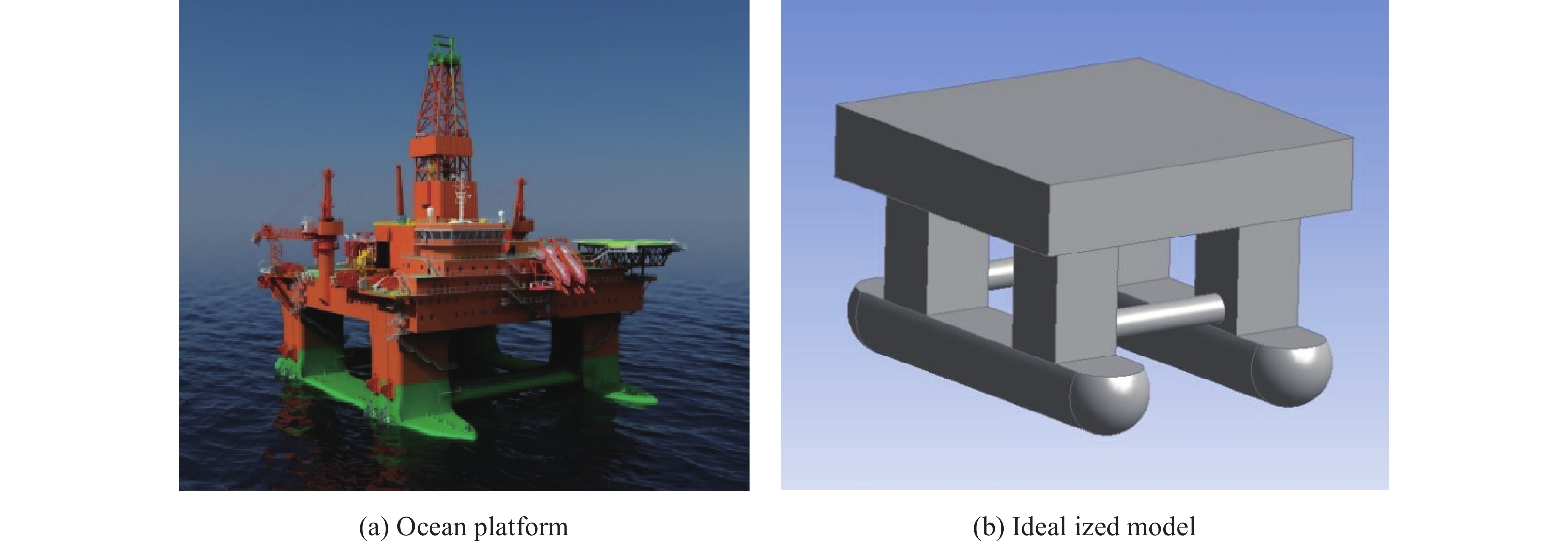
In general, the geometry of buoys, drilling rigs and ocean platforms can be idealized for simplicity in the construction of spheres, cylinders, and cube structures, as shown in Fig. 1, but until now there has been limited available data on their hydrodynamic coefficients. The aim of the present study is to explore the possibility of developing a numerical method to calculate the hydrodynamic coefficients for different shape structures such as spheres, cylinders, and cubes. A RANS approach is adopted here to obtain 3D hydrodynamic coefficients that include viscous and rotational flow effects as well as free surface wave generation.

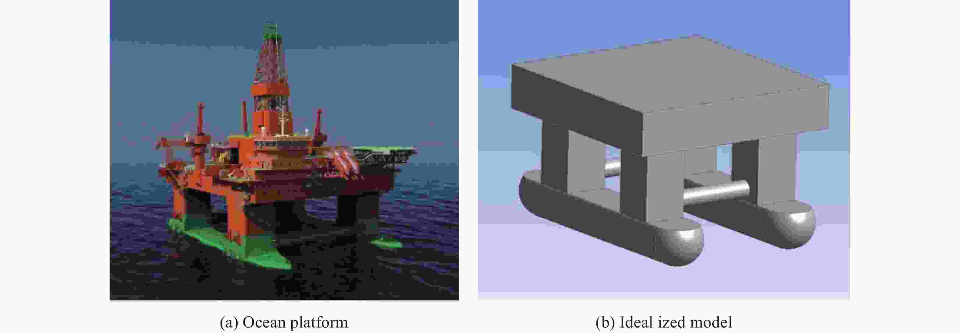
Figure 1.  Ocean platform and its idealized model

The viscous flow around the structure is governed by 3D, unsteady, incompressible RANS equations ^[23]:

Where:

$ {u_i} $ —— the time-averaged velocity components (m/s) in Cartesian coordinates $ {x_i}\left( {i = 1,\;2,\;3} \right) $;

$ \rho $ —— fluid density (kg/m³);

$ {F_i} $ —— body forces (N);

P —— the time averaged pressure (Pa);

$ \mu $ —— viscous coefficient;

$u_i^{'}$ —— the fluctuating velocity components in Cartesian coordinates (m/s);

$ - \rho \overline {u_i^{'}u_j^{'}} $ —— the Reynolds stress tensor.

The finite volume method is employed to discretize the governing equation with the second-order upwind scheme to improve the computational accuracy. The semi-implicit method for pressure-linked equations (SIMPLE) is used for the pressure-velocity coupling. In order to allow closure of the time-averaged Navier-Stokes equations, various turbulence models have been introduced to provide an estimation of $ - \rho \overline {u_i^{'}u_j^{'}} $. Here, the realizable $ k - \varepsilon $ model is chosen ^[28], as used for applications in a wide range of flows due to its robustness and economic merit, and the standard wall function is applied for better analysis of the turbulent viscous flow around the wall.

To capture the water air free surface, an Eulerian method termed the volume of fluid (VOF) method is adopted. The equation for the volume fraction is:

Where:

$ \alpha $ —— the volume fraction of water and ($ 1 - \alpha $) represents the volume fraction of air.

The volume fraction of each liquid is used as the weighting factor to obtain mixture properties such as density and viscosity, i.e.

Where:

$ {\rho _{\mathrm{w}} } $, $ {\rho _{\mathrm{a}}} $ —— the density of water and air (kg/m³);

${\mu _{\mathrm{w}}}$, ${\mu _{\mathrm{a}}}$ —— the viscosity of water and air (m/s).

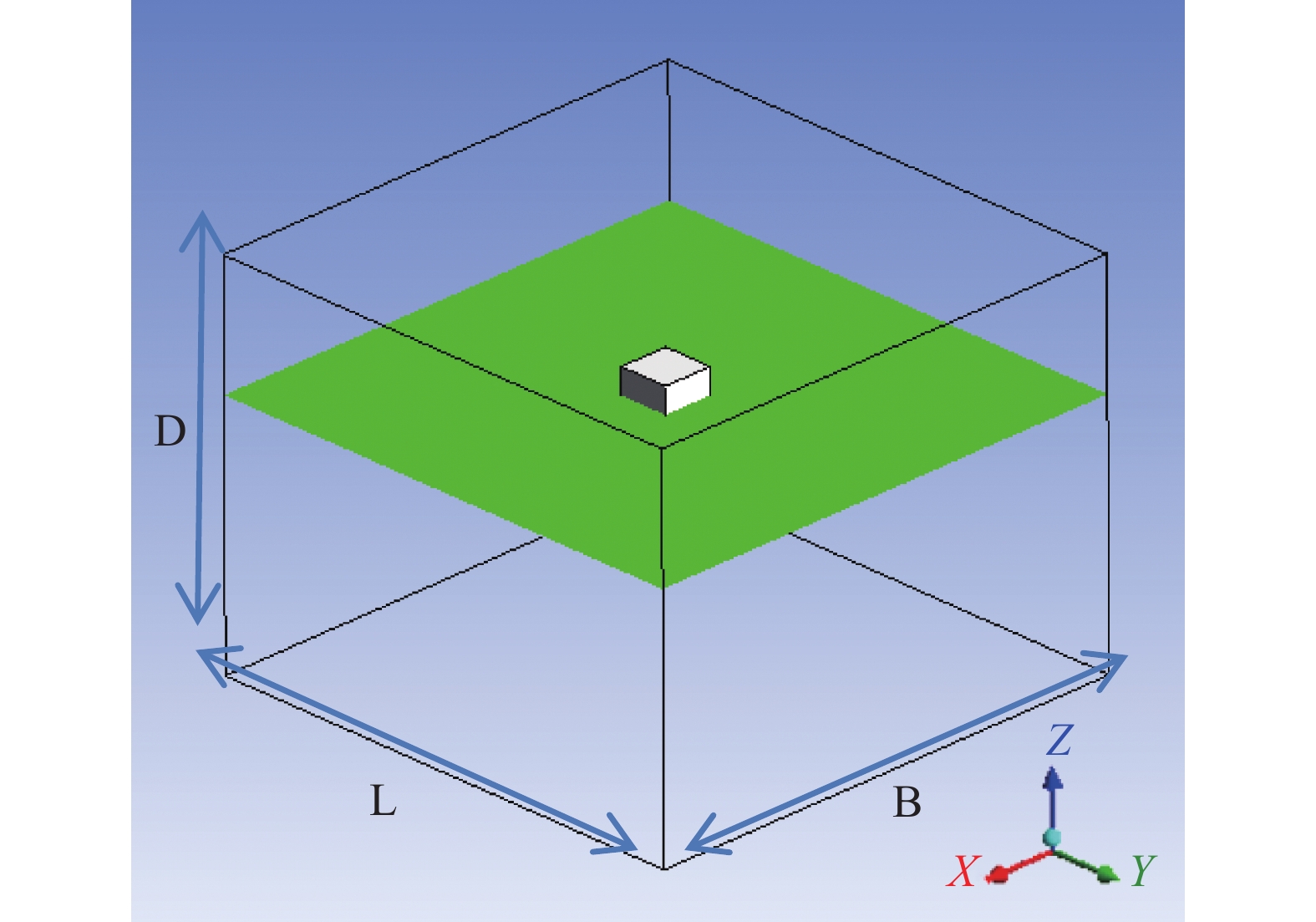
In the present study, the computational analysis incorporates three geometric models: a sphere, a cylinder, and a cube. Detailed specifications of these models, including dimensions, volume, and surface area, are systematically outlined in Tab.1. The calculation domain is −10 m < x < 10 m, −10 m < y < 10 m, −10 m < z < 5 m. The body-fixed coordinate system is defined with the origin precisely positioned at the center of the geometrical models. The geometry of the structure is shown in Fig. 2. Structures characterized by vertical sides and a flat bottom forms a significant category within marine engineering, attributed to their straightforward construction methodology and diverse utility, encompassing barges, pontoons, and offshore platforms. Here, the cube structure taken as a rigid body is shown as an example, where the region above the green interface signifies the gas phase, the region below it corresponds to the liquid phase, and the green interface itself demarcates the free surface.

Figure 2.  Computational domain for numerical simulation

The boundary conditions around the model are as follows: a wall boundary with a no-slip condition is applied to the bottom of the computational domain. The top and the surroundings of the computational domain set symmetry boundary conditions, a no-slip wall boundary condition is applied to the model to numerically simulate the oscillatory motion produced in the PMM tests, a user-defined function is employed to control the motion of the model, and the SIMPLE is used for the pressure-velocity coupling. The finite volume method is employed to discretize the governing equation with the second-order upwind scheme. The VOF method is adopted to capture the nonlinear free surface. For calculation of the cell surface flow, a more accurate method termed Geo-Reconstruct (from ANSYS 14.0) is applied. In the process of calculation, it is very important to determine the time step, as the curves of force and moment will zigzag because of oscillation of information when the time step is too small. On the other hand, errors such as negative volume and numerical divergence will occur if the time step is too large. After repeated testing, an adaptive time step has been determined. The method has high degree of precision and high computation speed and convergence when the time step is approximately equal to one 200th of the period.

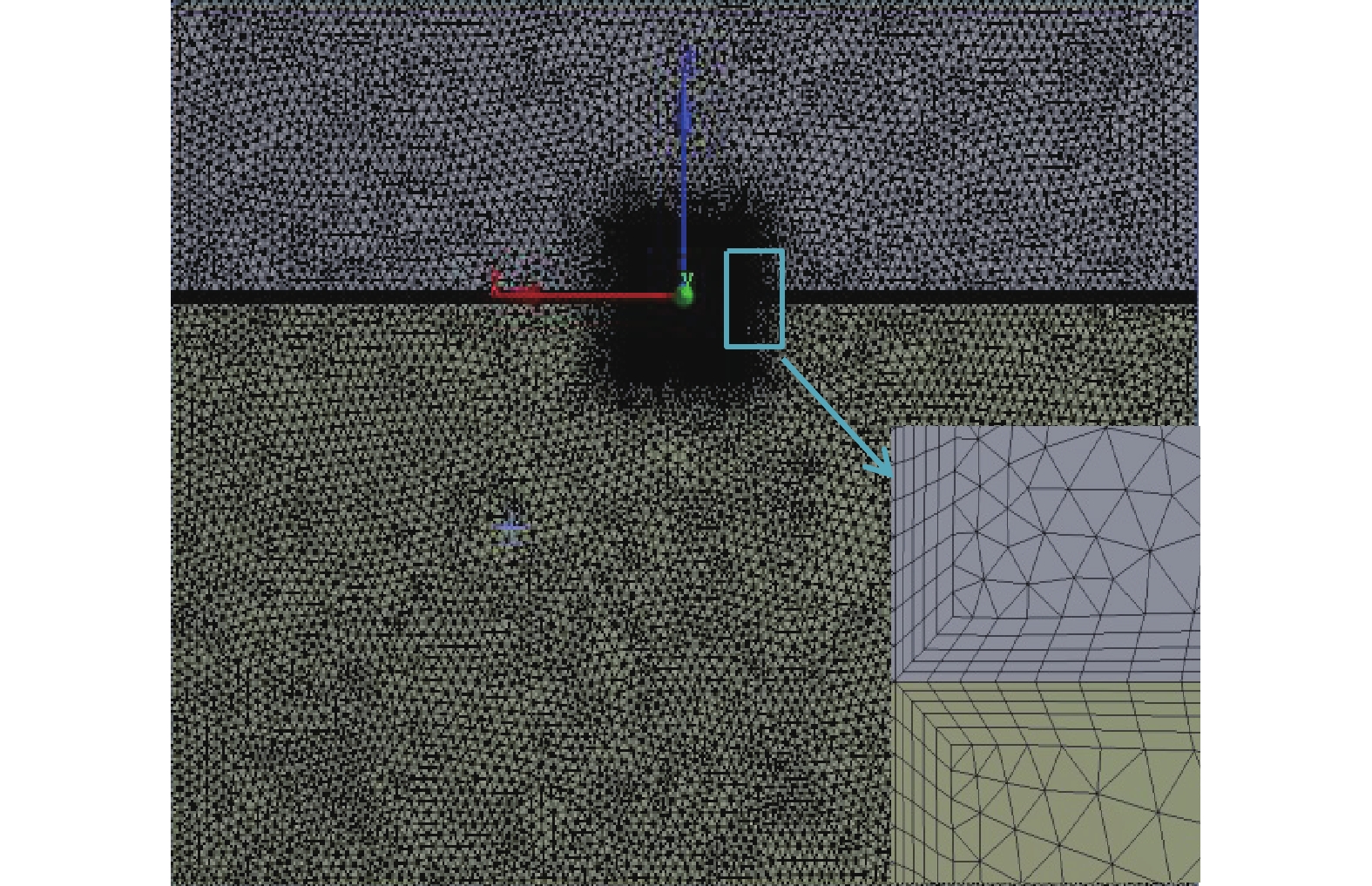
To simulate the motion of the model, the fluid domain is split into two regions, a boundary layer region and an outer region. The grid is generated by a hybrid mesh strategy: in the boundary layer region, a prism mesh is used to define the fluid surrounding the model, which permits detailed control of the mesh parameters and the element quality. The first node is positioned close enough to obtain an average periodic y+, which is the distance of the first node from the model in non-dimensional wall units. The unstructured tetrahedral mesh can be conveniently remeshed when element deformation is used in the outer region distant from the model, which is rather coarse, so the number of grids can be reduced, as shown in Fig. 3. In order to capture the wave surface accurately and calculate the force and moment acting on the structure precisely, the meshes in surface zones and zones along the body are refined as shown in Fig. 4. Numerical simulations are performed with the CFD software Ansys Fluent. All calculations are performed on a Dual 3.06 GHz 64 bit Opteron machine with 48.0 GB RAM. Typical time per computational time step is 2 min 3 s for a mesh size of 2.5 million cells.

Figure 3.  Meshes of computational area

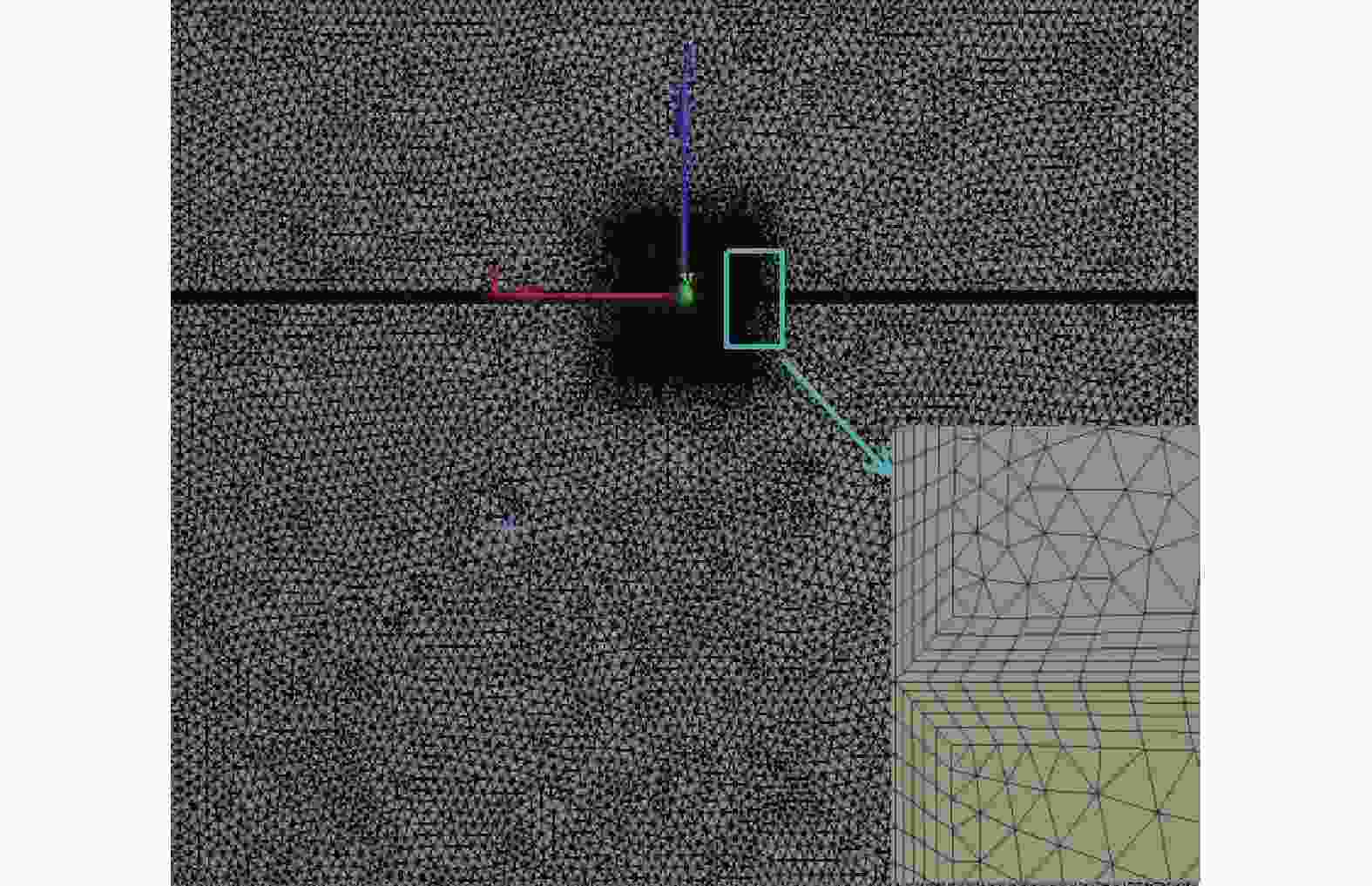
Figure 4.  Plane y=0 of computational area

Lin ^[29] selected different mesh sizes for independence analysis, which proved that the mesh size used had good convergence. The mesh size used in this paper was consistent with the literature. Therefore, this paper does not analyze grid independence.

The PMM generates two kinds of motion, translation and rotation, imposed on the structure. "Pure heaving", "pure swaying", and "pure rolling" are approximately sinusoidal motions in fluid dynamics. Thus, rotary-based and acceleration-based coefficients can be explicitly determined. The system is designed to obtain the hydrodynamic characteristics of ocean floating structures in either translation or rotation of motion.

The displacement of the model on the k-th mode is given by the following equations:

Where:

$ {x_{k0}} $ —— the amplitude of the motion (m or rad);

$ \omega $ —— the frequency of the motion (rad/s);

$ k = \{1,\;2,\;3,\;4,\;5,\;6\} $ —— surging, swaying, heaving, rolling, pitching, and yawing, respectively.

The normal force acting on the model can be described by the equations:

Where:

$ k,j = \{1,\;2,\;3,\;4,\;5,\;6\} $ —— surging, swaying, heaving, rolling, pitching, and yawing, respectively;

$ {\mu _{jk}} $, $ {\lambda _{jk}} $ —— added mass and damping of each mode;

$ {F_{jk}} $, $ {M_{jk}} $—— hydrodynamic force and moment.

In fact, the theoretical normal force acting on the model is the integral of the surface discrete element stress. The model surface pressure $ p $ includes dynamic pressure $ {p_{\mathrm{d}}} $ and static pressure $ {p_{\mathrm{s}}} $. The static pressure of the grid cell is $ {p_{\mathrm{s}}} = \left\{ \begin{gathered} 0\;\;\;\;\;,\;{x_3} \geqslant 0 \\ - \rho g{x_3},\;{x_3} < 0 \\ \end{gathered} \right. $ so the dynamic pressure on the grid cell $ {p_{\mathrm{d}}} = p - {p_{\mathrm{s}}} $. The theoretical dynamic force $ {F_k} $ on the k-th direction acting on the model is the integral of the surface $ {S_0} $ discrete element stress, so $ {F_k} = \displaystyle\int\limits_{{S_0}} {{p_{\mathrm{d}}}{n_k}{\mathrm{d}}s} $, where k is the x, y, and z direction respectively; the rolling moment can be expressed as $ {M_4} = \displaystyle\int\limits_{{S_0}} {{p_{\mathrm{d}}}({r_2}{n_3} - {r_3}{n_2})} {\mathrm{d}}s $ accordingly, where $ {n_2},\;{n_3} $ are the unit weight of the normal direction. $ {r_2},\;{r_3} $ are the y and z component of the distance between the center of the discrete cell element and the model rotation center. For simplicity, the mode of operation applied to a submarine in the vertical plane is discussed here.

During pure heaving motion, the models of vertical displacement, velocity, and acceleration are given by the following equations:

The normal force acting on the model during pure heaving motion can be described by the equations:

Using the least squares method to fit the curve of force and moment acting on the hull during the pure heaving test, so:

F₃₀ —— the error between the CFD software fluent calculation of hydrostatic values and the user-defined function program to calculate the hydrostatic values, the error is caused by p_s calculation;

M₅₀ —— the error of the moment caused by p_s calculation;

F_3A, F_3B, M_5A, M_5B —— the amplitudes after the least square method fitting.

Special note is taken that the existence of F₃₀ and M₅₀ does not affect F_3A, F_3B, M_5A, M_5B.

When the Eq. (9), Eq. (10), and Eq. (13) are plugged into Eq. (11), in order to make the equation coefficient of both sides equal, the added mass and damping of the heaving motion at the frequency equal to ω are given by the following equation:

Accordingly, when the model is a "pure" heaving motion, we can obtain the added mass and damping of the heaving and the coupling of heaving and pitching; the added mass and damping of 6 DOF (including the coupling added mass and damping of each degree) can be obtained by this method.

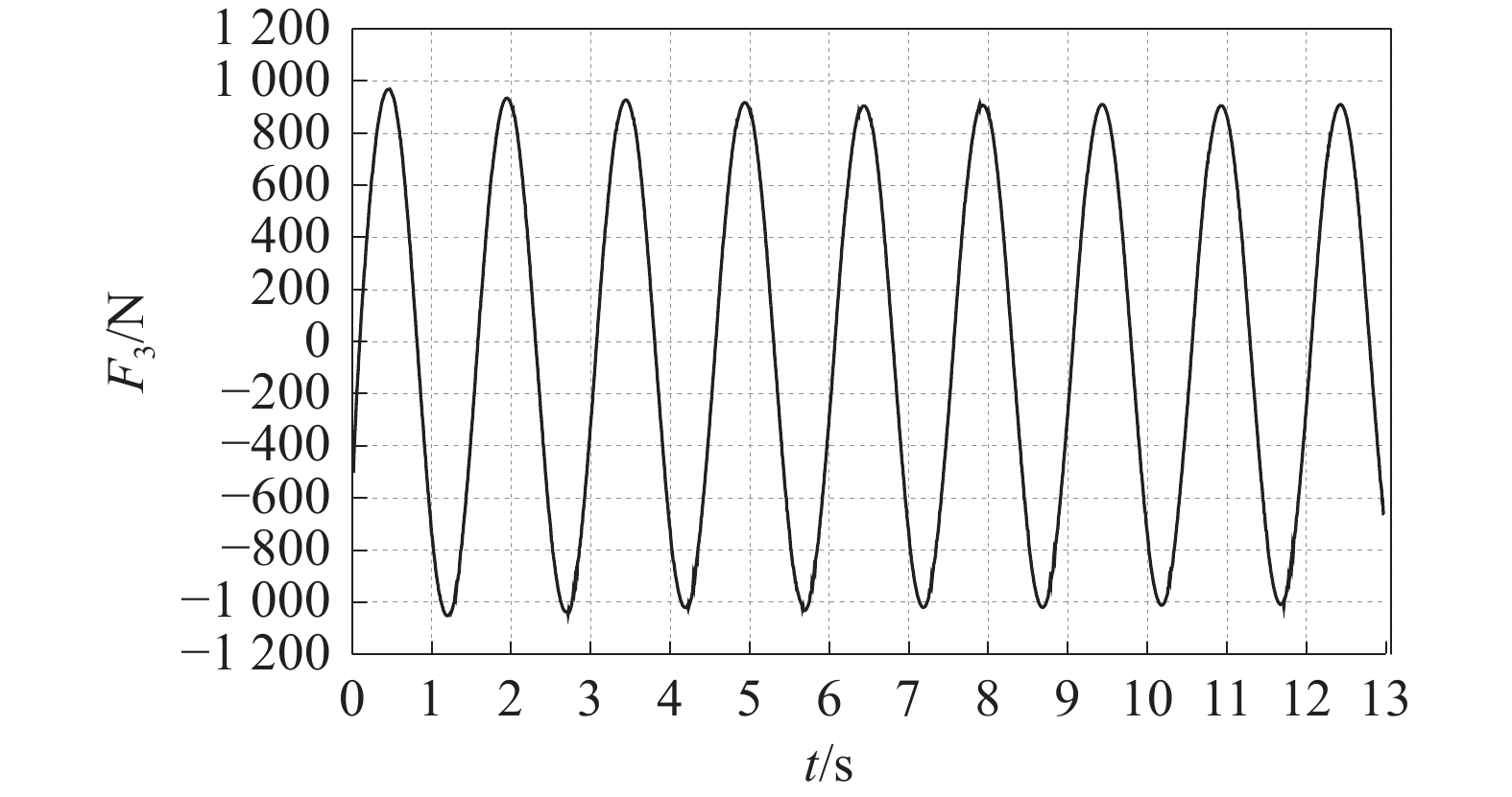
In this section, comprehensive numerical analyses are conducted on three distinct geometric models: a sphere, a cylinder, and a cube. The cube is specifically utilized as a case study to elucidate the methodology for determining the added mass and damping coefficients. The analysis employs a forced oscillation approach, where the cube undergoes oscillation at a constant frequency and amplitude in a single mode. This simulation enables the precise calculation of the cube's added masses and damping coefficients in response to heave, surge, and roll motions in a quiescent water environment. The computational framework for these determinations is grounded in the detailed simulation of the flow field around the structure. As shown in Fig. 5, the heave force oscillates at the period given when the period of the cube oscillation is 1.5 s, the amplitude of displacement is 0.02 m and, with the imposed harmonic displacement in heave, x₃=0.02sin2πt, the computed time history of the cube heave force of heave motion is presented. According to Eq. (11), the least square method is applied to fit the hydrodynamic force and moment time histories, as for the curve in Fig. 5, F₃=942.7sin(2π/1.5t)−243.3cos(2π/1.5t)−45.14. The results obtained are F_3A=942.7, F_3B=−243.3, ω=2π/1.5 and F₃₀=−45.14. Clearly, the error is only about 0.11% of the hydrostatic value, and with the error value 45.14 N and the hydrostatic value of the cube 40.221 kN, the error is almost negligible. According to Eq. 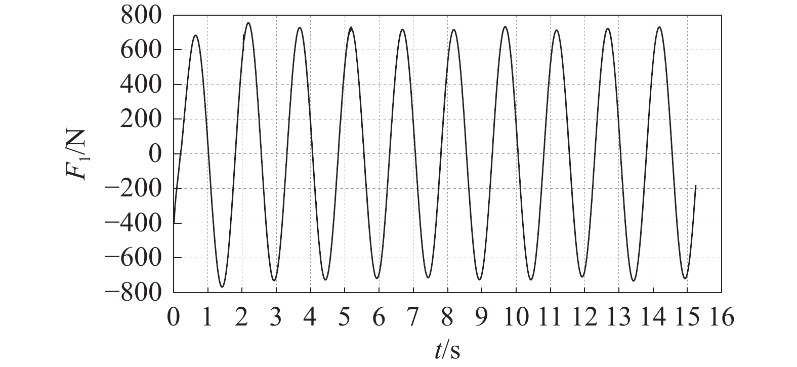(13), the added mass and damping of the heave motion are obtained as A₃₃=2686.37 kg and B₃₃=2904.18 N·s/m. As shown in Fig. 6, the computed time history of the cube surging force of surging motion is presented with the period of the oscillation 1.5 s, the amplitude of displacement 0.02 m, and the imposed harmonic displacement in surge of x₁=0.02sin2πt. A similar process can be used for added mass and damping for surge and roll, and then we can obtain the results of added mass and damping of surging motion with A₁₁=624.08 kg and B₁₁=8167.04 N·s/m. In Fig. 7, the computed time history of the cube roll moment of roll motion is presented with the period of the oscillation 1.5 s, the amplitude of roll displacement 0.01 rad, and the imposed harmonic displacement in roll, x₄=0.02sin2πt. The same method can be used to obtain the added mass and damping of rolling motion of A₄₄=679.93 kg·m and B₄₄=2478.04 N·s.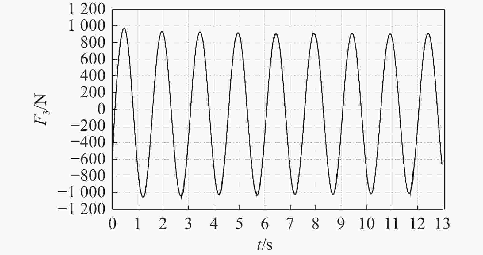

Figure 5.  Cube heave force of heave motion (T=1.5 s)

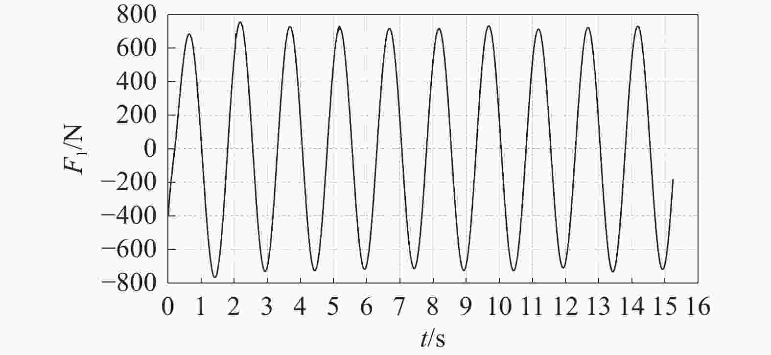
Figure 6.  Cube surge force of surge motion (T=1.5 s)

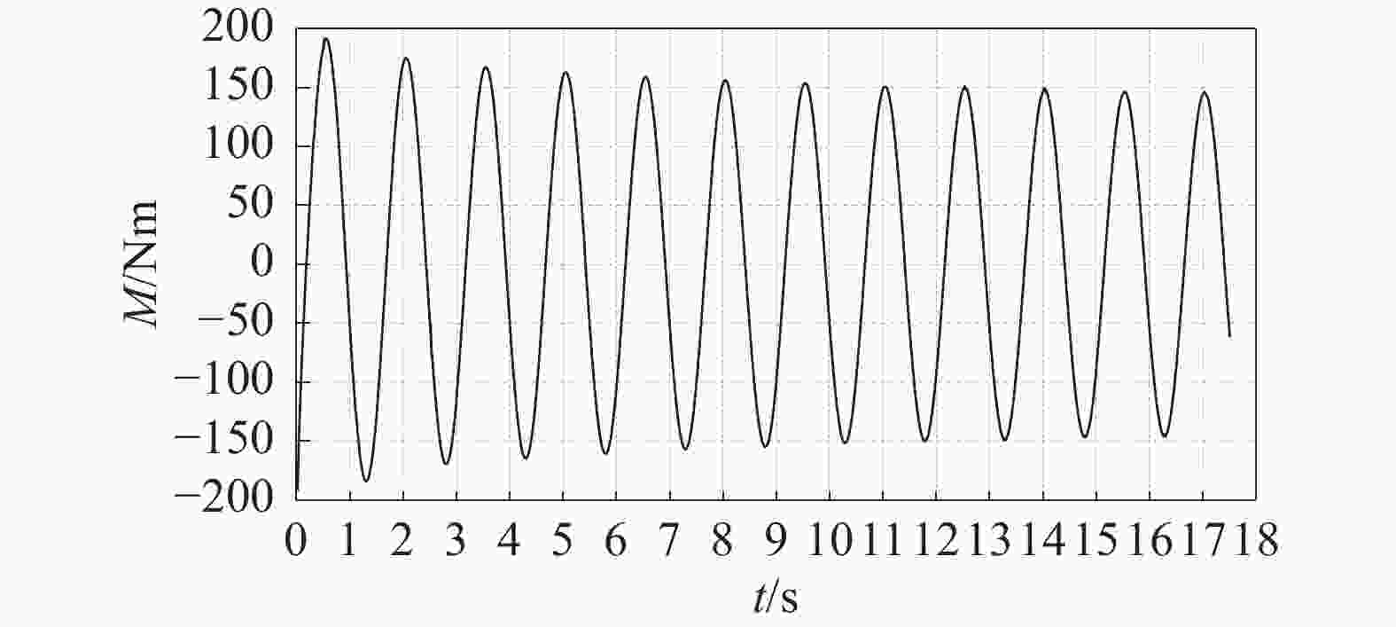
Figure 7.  Cube roll moment of roll motion (T=1.5 s)

Utilization of dimensionless equations confers a higher degree of generality upon the analytical framework, as these equations are invariant across different unit systems. This universality ensures that irrespective of the unit system employed, the application of a given dimensionless equation remains consistent. The transition to a dimensionless paradigm facilitates the reduction of complex, multivariable problems into more manageable forms characterized by fewer dimensionless parameters. Such simplification enhances the ease and intuitiveness of comparisons across systems that may vary in scale or operational conditions. The core of this methodological approach involves the synthesis of principal variables into dimensionless groups. Subsequently, these groups are employed to reformulate the equations or models pertinent to the investigation, thereby casting them in a dimensionless context.

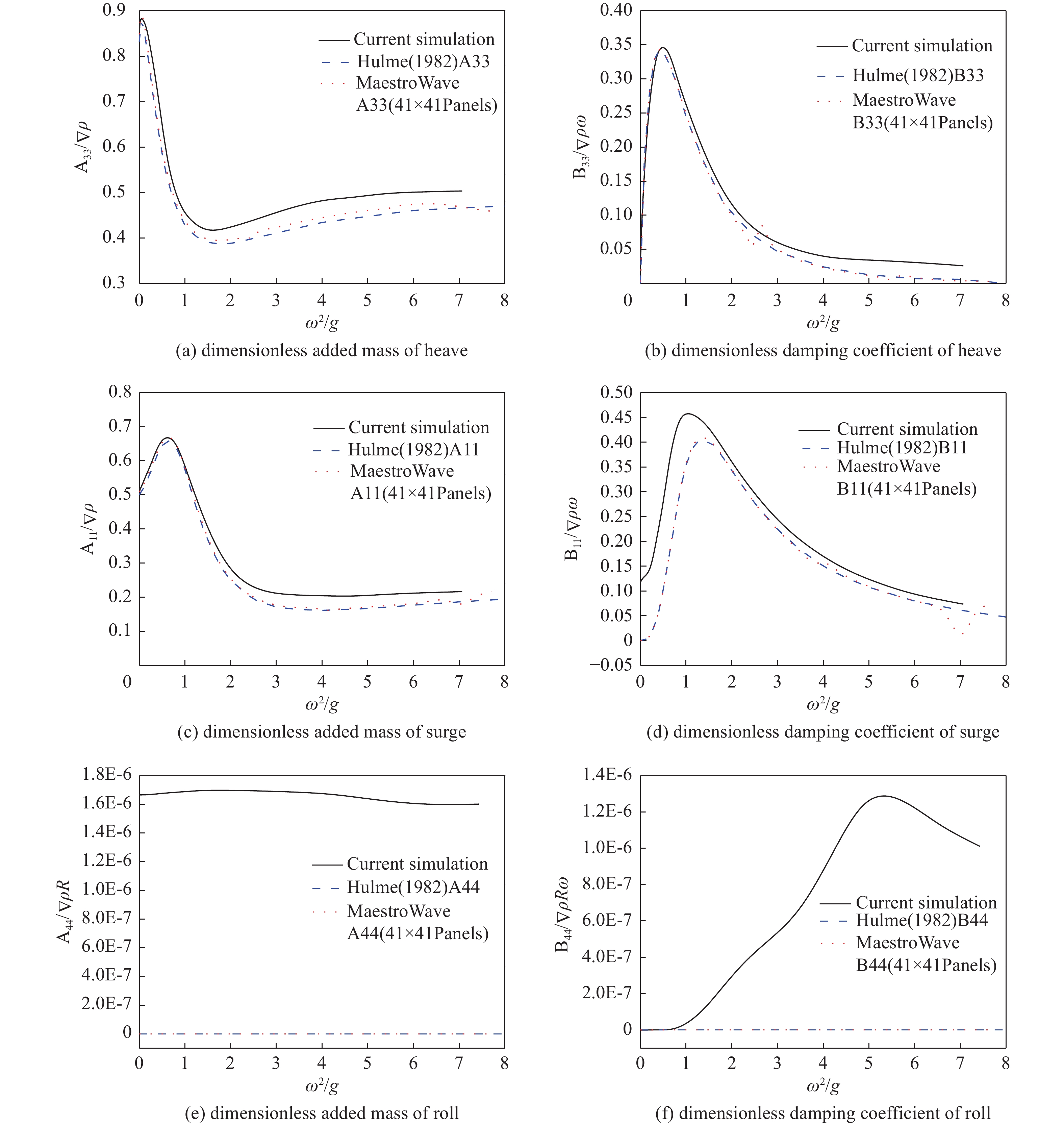
Fig. 8(a) and Fig. 8(b) are dimensionless added mass and damping coefficients of heave motion, respectively. The sphere is forced to heave and surge harmonically with 0.02 m of amplitude, respectively, and to roll harmonically with 0.1 rad of amplitude at the free surface. Fig. 8 shows the results of dimensionless hydrodynamic coefficients when the sphere heaves in calm water. It can be seen that the results obtained by the CFD method are in good agreement with those obtained by Hulme ^[30] and those obtained by the 3D surface source potential flow calculation software (which does not consider viscosity and nonlinear effects in the calculation) from the Advanced Marine Technology Center, DRS Technologies. It also can be seen that the dimensionless added mass and damping coefficients are greater than the results of potential flow theory at high frequencies; it seems that the results affected by high frequencies are more sensitive than those at low frequencies.

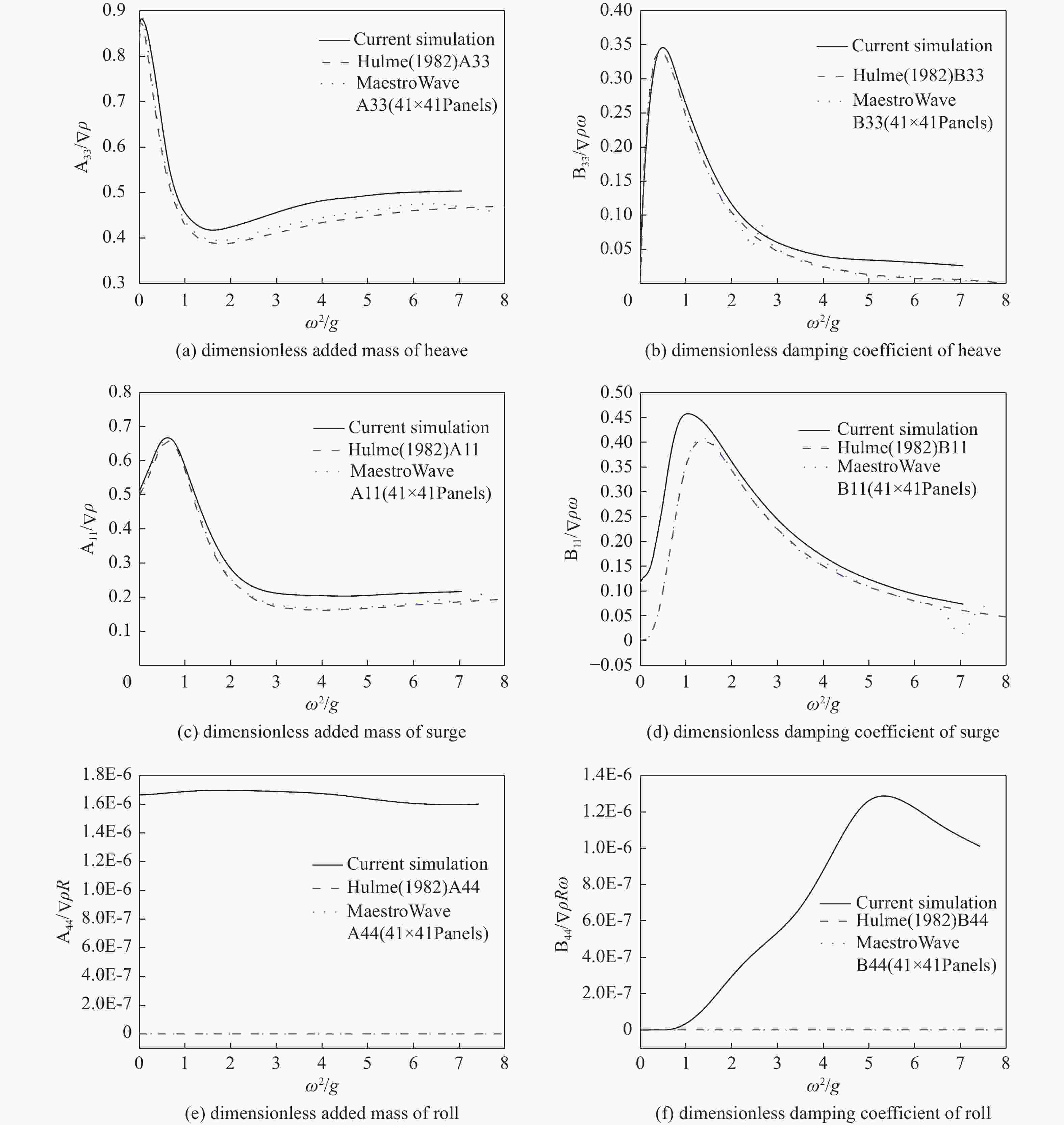
Figure 8.  Dimensionless added mass and damping coefficients for a sphere heaving, surging, and rolling in calm water

Fig. 8(c) and Fig. 8(d) are the dimensionless added mass and damping coefficients of surge motion, respectively. They give the hydrodynamic coefficients for the sphere surging in calm water. It can be seen that the added mass obtained by the CFD method agrees well with other methods: at high frequencies, the added mass is greater than the results obtained by potential flow theory, whereas at low frequencies, the damping coefficient is greater than results of those curves. Compared with the low-frequency situation, the effect of viscosity on the increment of added mass is more obvious at high frequencies.

Figs.8(e) and Figs.8(f) are the dimensionless added mass and damping coefficients of roll motion, respectively. They illustrate the hydrodynamic coefficients for the sphere structure rolling harmonically with 0.1 rad of amplitude about the center of the sphere in calm water, which was also subject to experimentation by Vugts ^[31] and the Advanced Marine Technology Center, DRS Technologies.

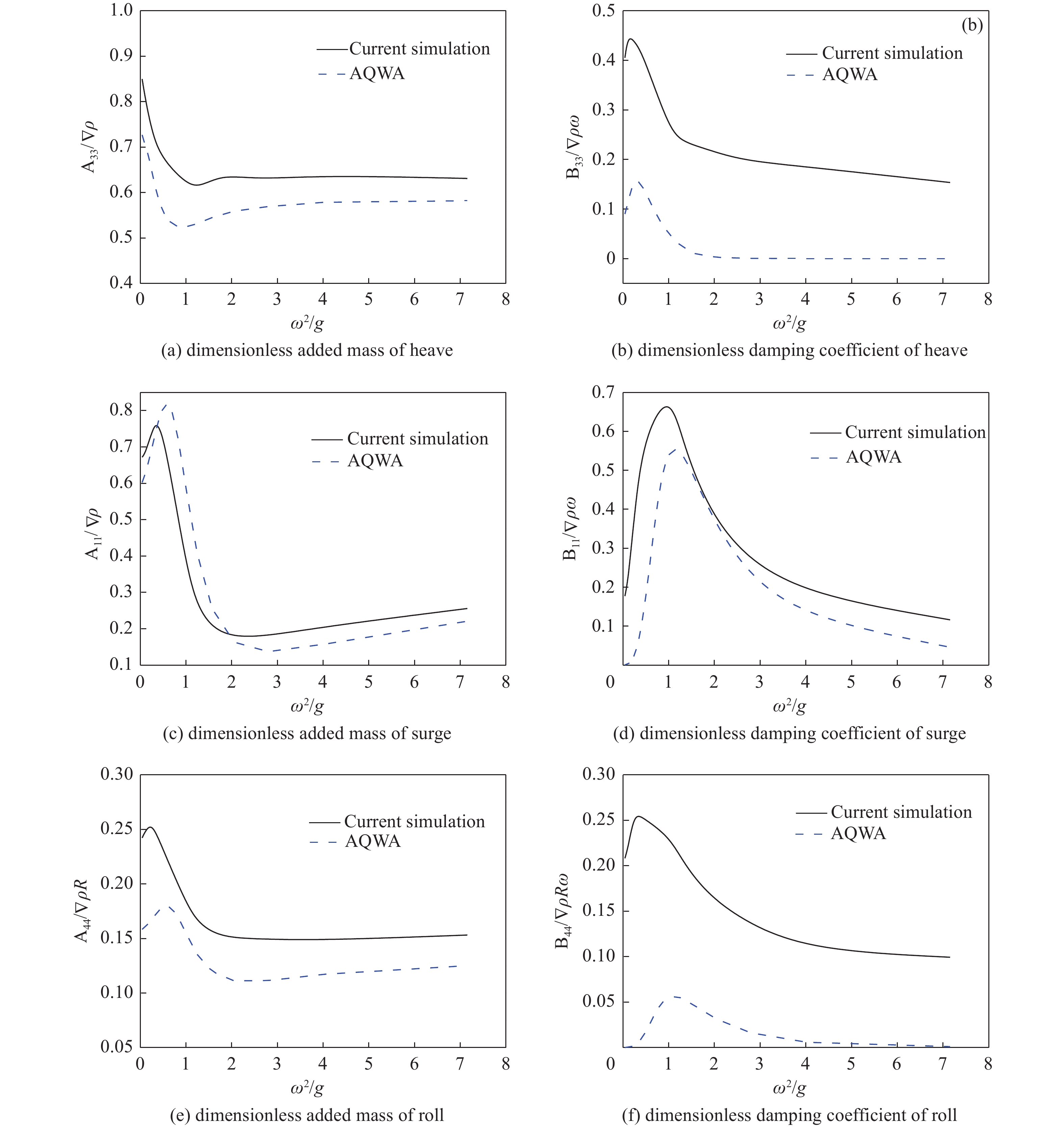
The hydrodynamic properties of a vertical circular cylinder as a function of ${\omega ^2}/g$ are shown in Fig. 9. The solid line represents the result of the current prediction and the dashed line represents the result obtained by AQWA software, which is based on potential flow theory. No experimental data is available from model tests.

Figure 9.  Dimensionless added mass and damping coefficients for a vertical cylinder heaving, surging, and rolling in calm water

The vertical cylinder oscillates at the free surface in three typical models heaving, surging, and rolling. The period of oscillation varies from 0.75 s to 10 s. The amplitudes of heave and surge motion are the same, 0.02 m, and the amplitude of roll motion is 0.01 rad. The results show a good agreement between the current CFD method and the AQWA simulation, indicating the CFD approach is reliable for this type of analysis.

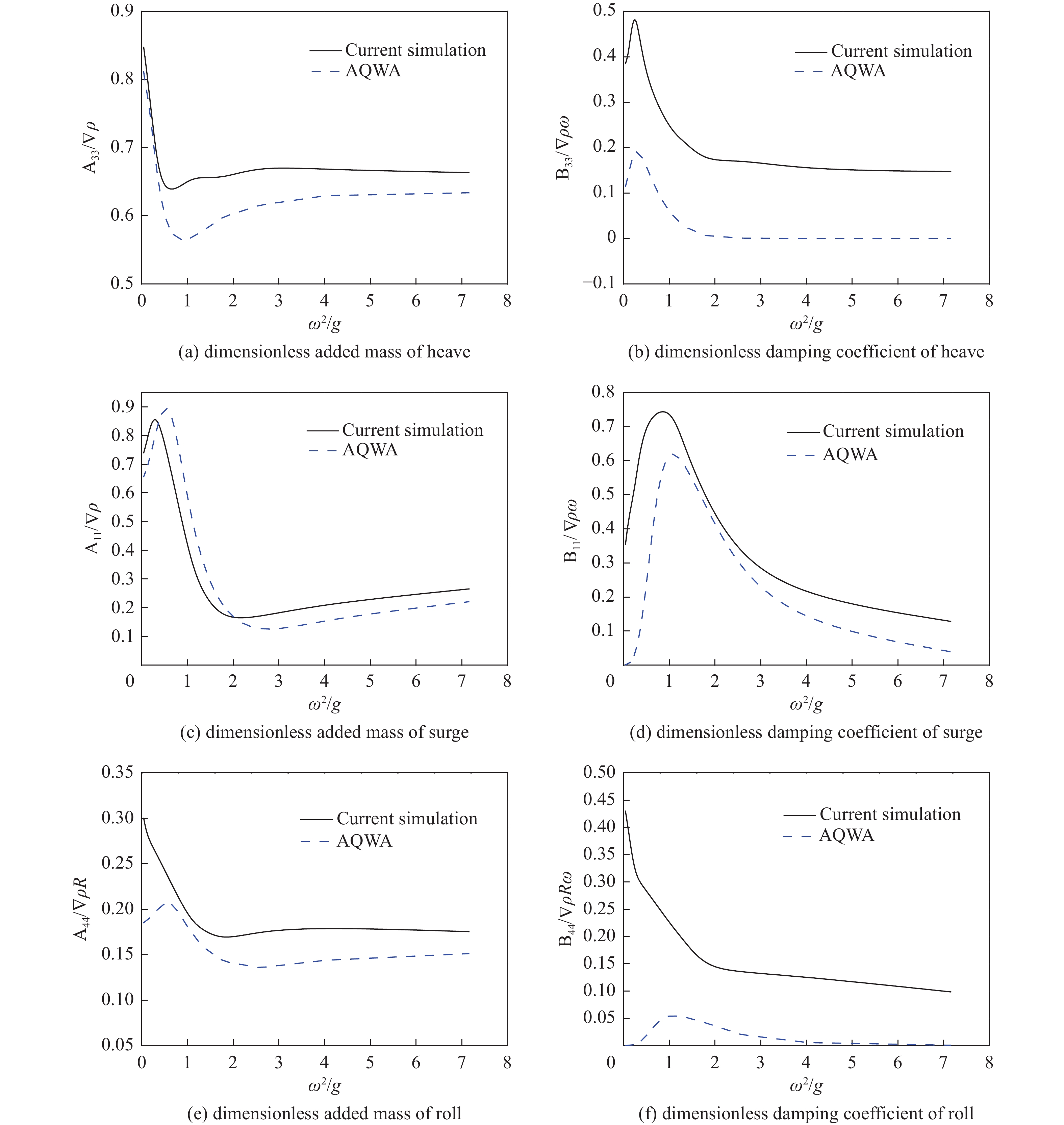
A cube harmonically heaving, surging, and rolling at a free surface is studied. The working condition is the same as in the previous cylinder case. The current method, using the hybrid mesh shown in Fig. 3 and Fig. 4, is thus compared with the potential flow results obtained by using the AQWA software. Dimensionless added mass and damping coefficients for a cube heaving, surging, and rolling in calm water are represented in Fig. 10.

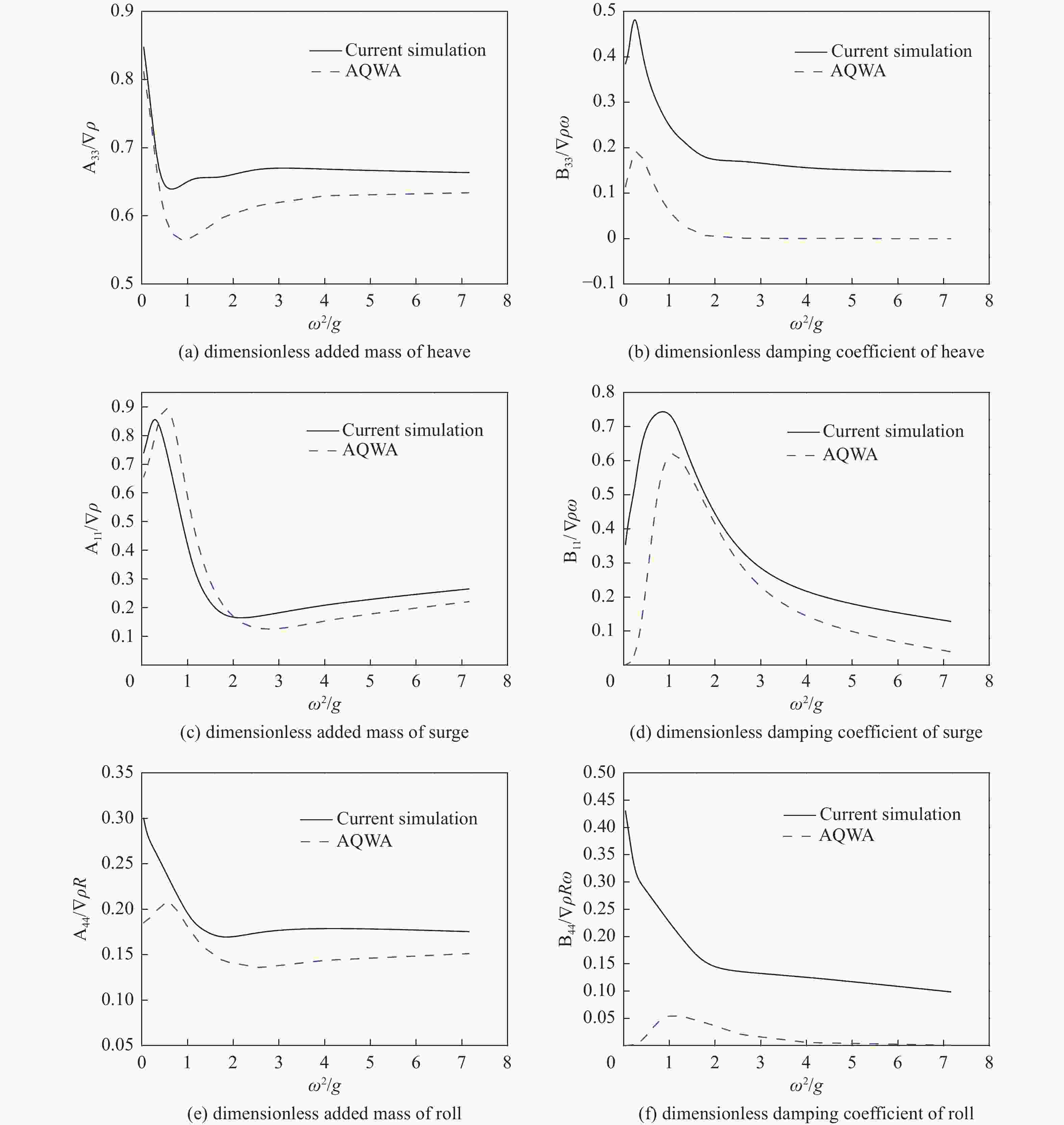
Figure 10.  Dimensionless added mass and damping coefficients for a cube heaving, surging, and rolling in calm water

In summary, the observed trends are markedly evident; the RANS (Reynolds-Averaged Navier-Stokes) simulations pertaining to the dynamics of the models yield superior outcomes in comparison to those derived from the theoretical potential flow solution, with particular emphasis on the rolling mode. The analysis of the results across the three cases reveals consistent phenomena. From Fig. 8(d), Fig. 9(d), and Fig. 10(d), the damping coefficient is greater than the results of those curves at all frequencies. The largest difference between two results appears near $ \omega $²/g=1. From Fig. 9(b), Fig. 9(d), and Fig. 9(f), our research shows that viscosity causes higher damping, which is to be expected. This phenomenon was also reported by Vugts ^[31]. From Figs.8(f), Fig. 9(f), and Figs.10(f), some discrepancies are noted, the reason being that the damping of roll is heavily determined by fluid viscosity which is not taken into consideration by potential flow theory. Consequently, a marked difference between the results of this CFD method and potential flow theory is evident. The method used in this research with the viscosity effect considered can predict the results more reasonably. Obviously, the current simulation method for solving this problem is more accurate.

It also can be seen that the dimensionless added mass and damping coefficient are greater than the results obtained by AQWA at all frequencies, especially the damping coefficient shown in Figs.9(b) and Fig. 10(b). Compared with the agreement between the CFD method and potential flow theory in the sphere case shown in Fig. 8(b), what makes such a huge difference here is that the viscous flow related to the real flow is governed by the complex motion of vortices at the sharp corners of the cylinder. Unlike the smooth transitions of shape of the sphere, cylinder, and cube, which have the same shape characteristics, vertical-sided objects with a flat bottom create serious vortices. Those shape characteristics of sphere, cylinder, and cube also lead to major differences in potential flow values in Fig. 8(e), Fig. 9(e), and Fig. 10(e), by using potential flow theory the added mass and damping of sphere's roll almost equal to zero while obvious variation trends of potential flow values are observed in Fig. 9(e) and Fig. 10(e), the dimensionless added mass of cylinder and cube rolling in calm water. On the other hand, when the flow field around the cylinder is analyzed by potential flow theory, the effect of the cylinder boundary layer interaction due to fluid viscosity is neglected.

From the above comparisons, we conclude that at both low and high frequencies, the trend of curves between the CFD results and potential flow theory is consistent in the case of heaving and surging, but the current method reflects the effect of viscosity, more in line with the actual situation. Among other causes of difficulty, roll characteristics are inherently difficult to measure because of the large mass inertia and hydrostatic moment; consequently, one of the most important advantages of the current method is that it predicts the added mass and damping of rolling, whereas potential flow theory cannot reach an accurate solution.

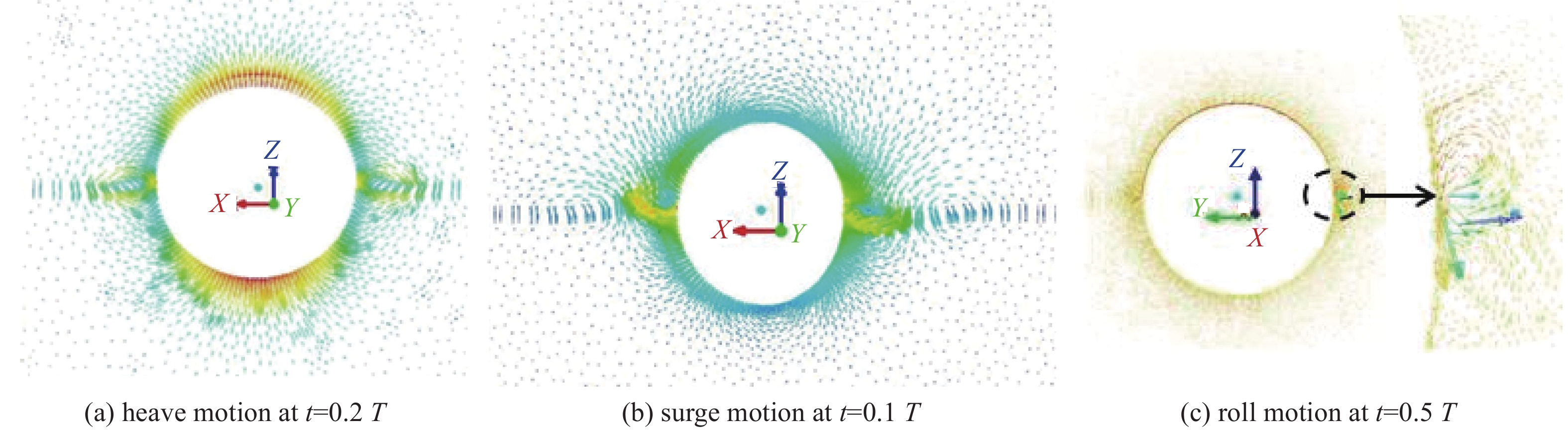
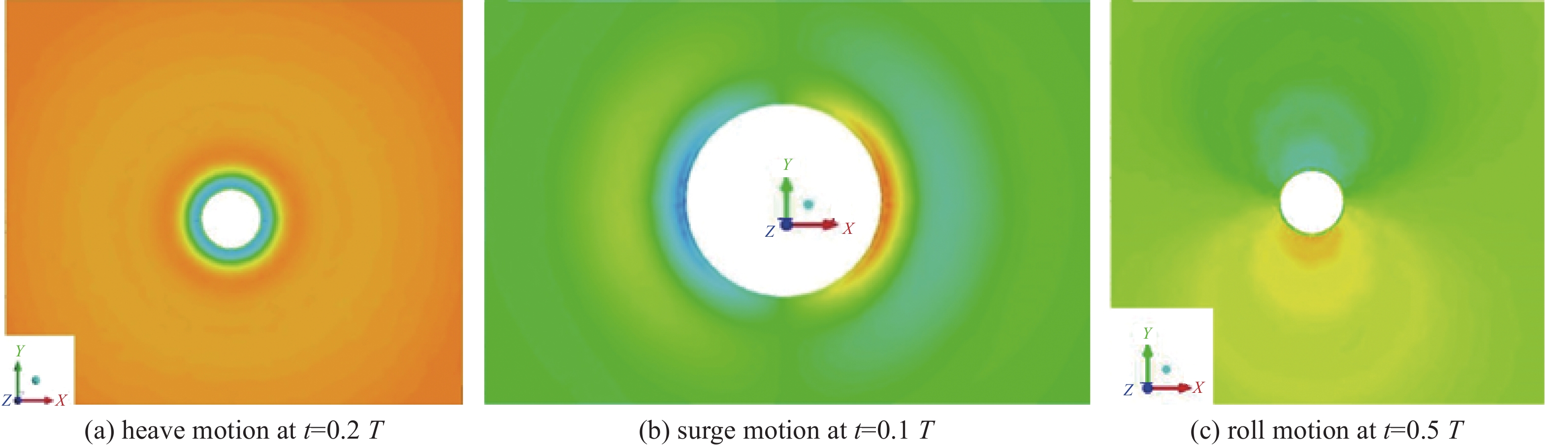
This section briefly presents simulation results of the velocity vector graph of flow field and free surface in the case of a sphere. Fig. 11 shows a velocity vector graph of flow field for a sphere heaving, surging, or rolling in calm water. The vortices induced by these three typical motions on a sphere are observed clearly in Fig. 11, where there are obvious vortices on both left and right sides of the sphere for heaving (Fig. 11(a)) and surging (Fig. 11(b)). For rolling, local vortices can also be captured using local amplification as shown in Fig. 11(c). These all produce vortex damping, reflecting the complexity of the flow field. Near the border of the sphere, the velocity vector is slightly greater than in other regions in Fig. 11. This is due to the presence of fluid viscosity, which causes the motion of fluid near the sphere to harmonize with the process of periodic movement when the sphere moves, thereby increasing the damping of viscosity. This analysis clearly explains why the CFD results shown in Fig. 8(b), Fig. 8(d), and Fig. 8(f) are greater than the potential flow results. The production of vorticity and the position of the vortex core have a large impact on fluid damping. It is important to note that a related nonlinear phenomenon like a vortex influences the results of calculation of the hydrodynamic coefficient. Fig. 12 shows contour graphs of the free surface for a sphere heaving, surging, and rolling in calm water. The free surface elevation around the models can be clearly distinguished.

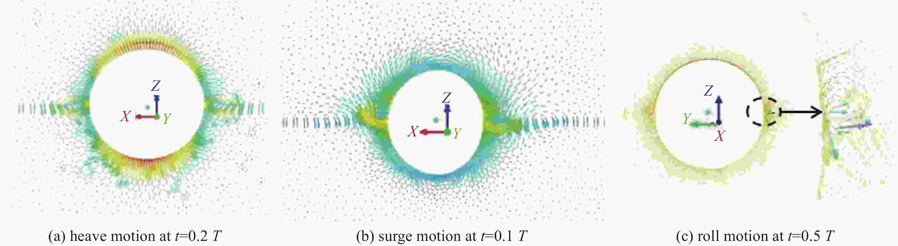
Figure 11.  Velocity vector graphs of flow field for a sphere heaving, surging, and rolling in calm water

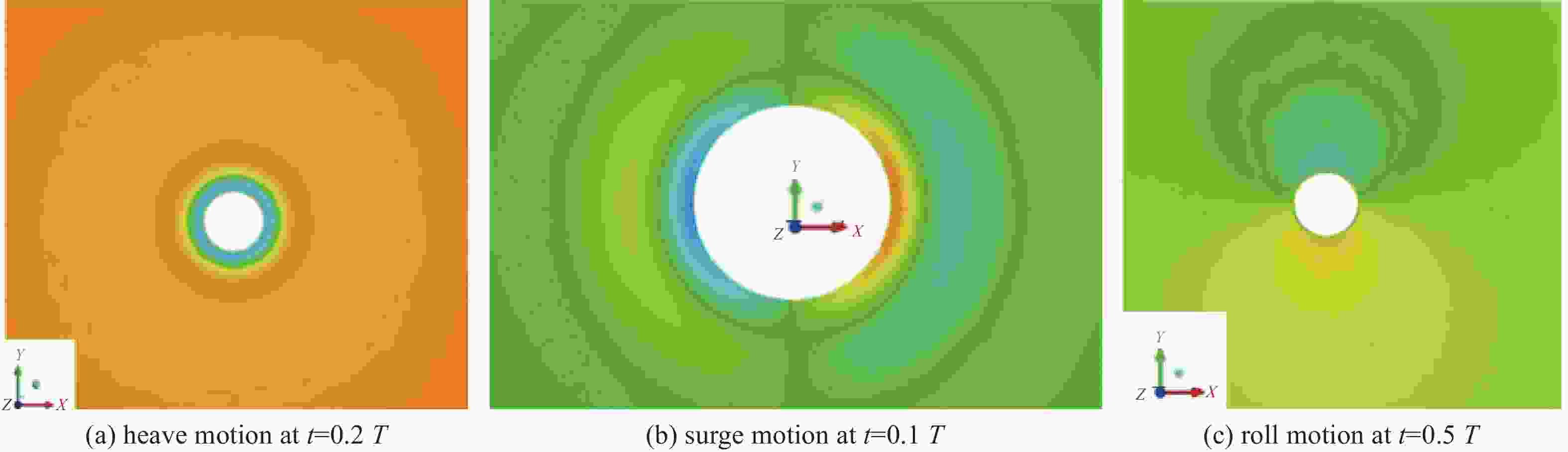
Figure 12.  Contour graphs of free surface for a sphere heaving, surging, and rolling in calm water

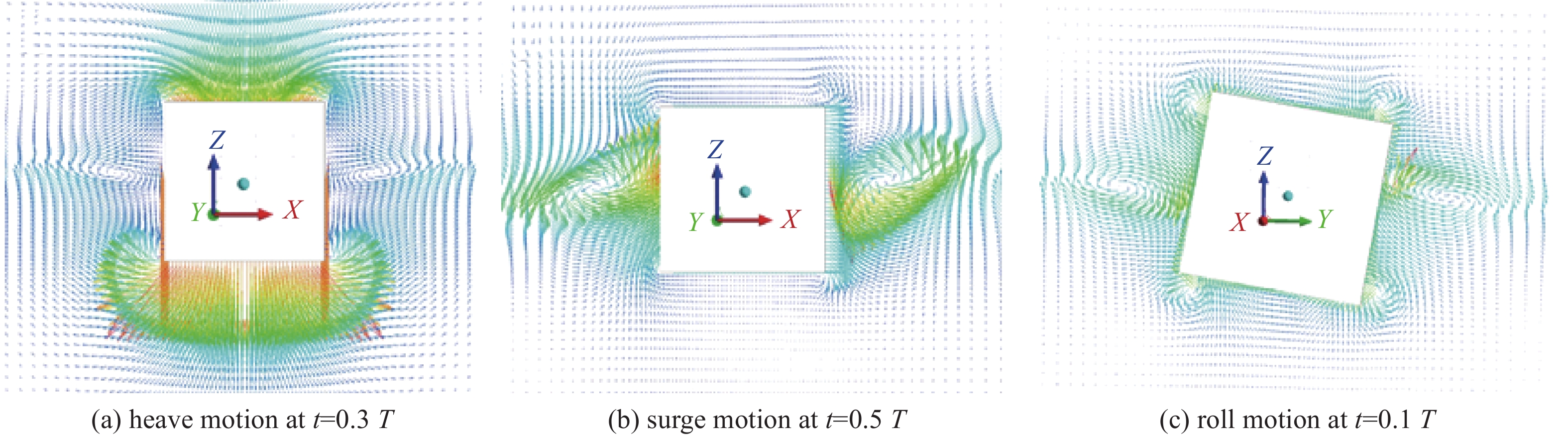
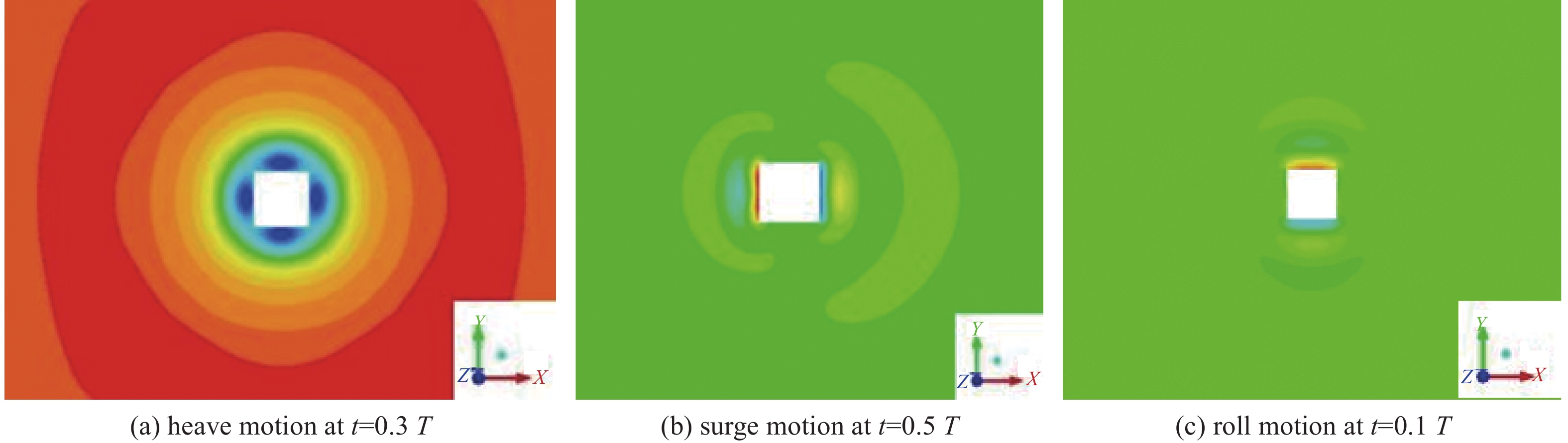
Velocity vector graphs of the flow field for a vertical cylinder heaving, surging, and rolling in calm water are shown in Fig. 13. The flow is governed by the complex motion of vortices at the sharp corners of the cylinder. As the cylinder starts to roll, an adverse pressure gradient develops immediately downstream of the corner, thereby causing a vortex. Fig. 14 shows contour graphs of the free surface of a cylinder heaving, surging, or rolling in calm water. The differentiated information about free surface elevation is well visualized.

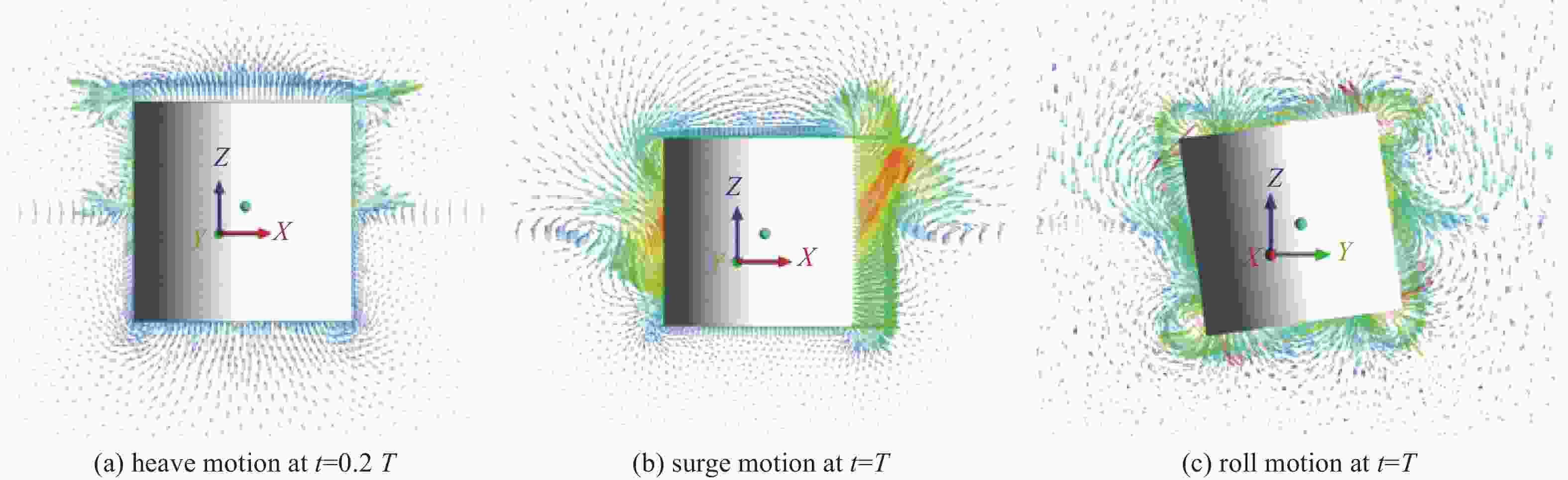
Figure 13.  Velocity vector graphs of flow field for a cylinder heaving, surging, or rolling in calm water

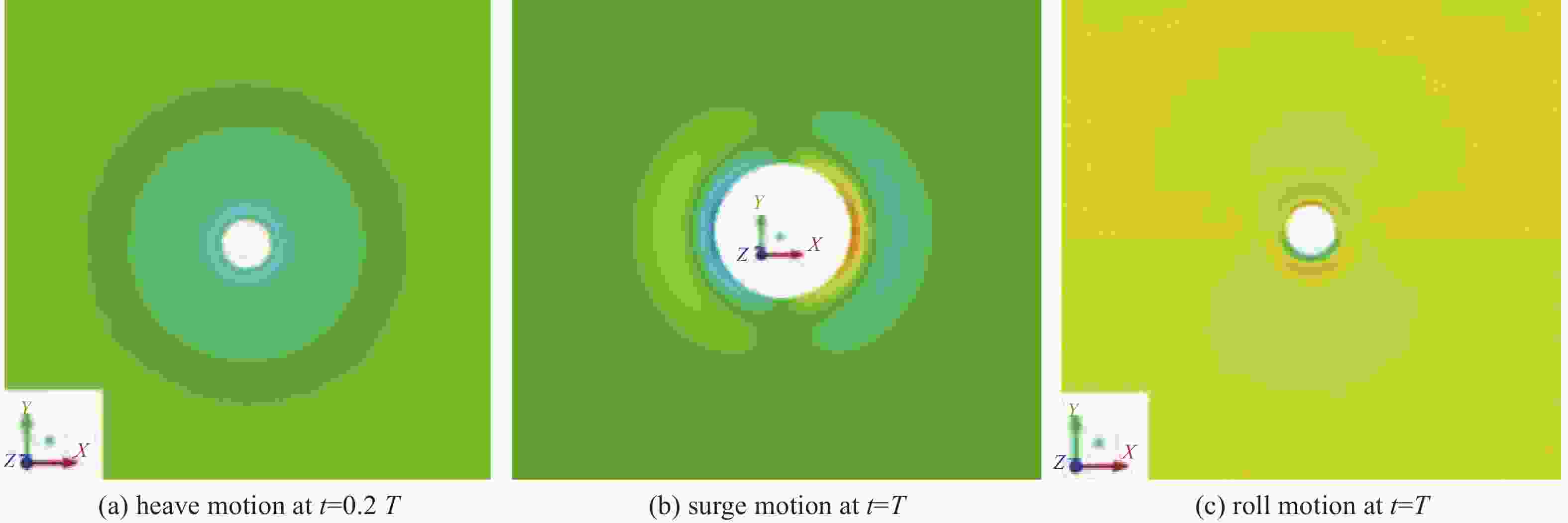
Figure 14.  Contour graphs of free surface for a cylinder heaving, surging, or rolling in calm water

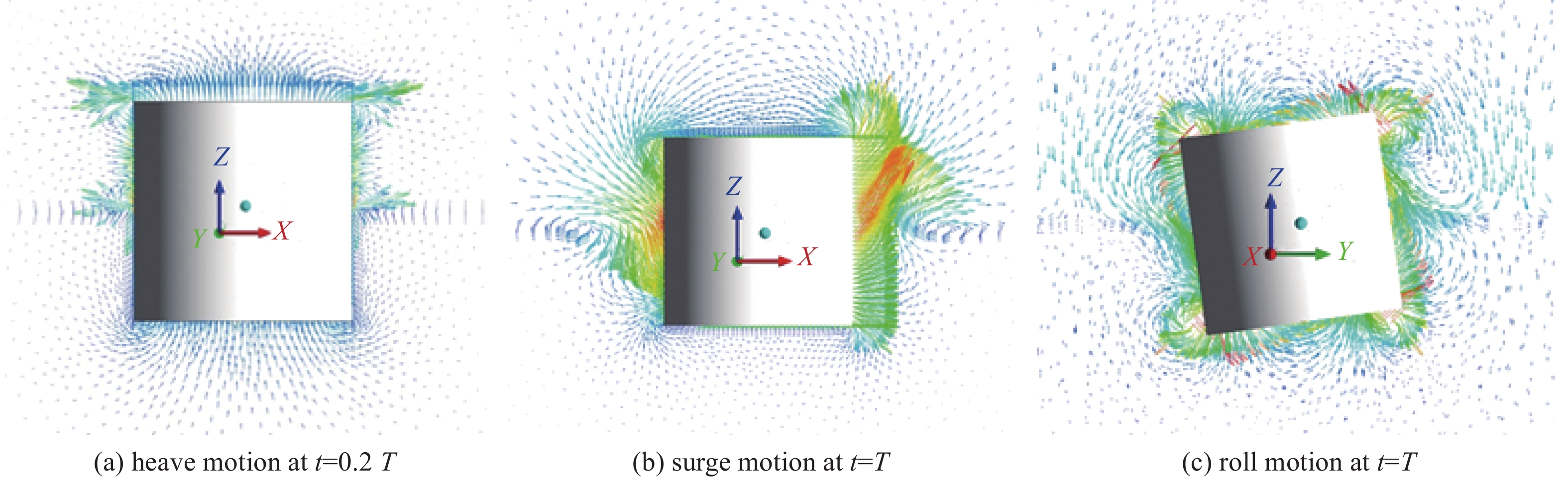
Fig. 15 shows velocity vector graphs of the flow field for a cube heaving, surging, or rolling in calm water. The process of analysis is similar to that for the previous cylinder case. Fig. 16 shows contour graphs of the free surface for a sphere heaving, surging, or rolling in calm water. The accurate capture of this complex flow is essential for accurate modeling of the fluid damping coefficient. This work indicates that not only are forces and moments well predicted, but the patterns associated with such flows are also well reproduced.

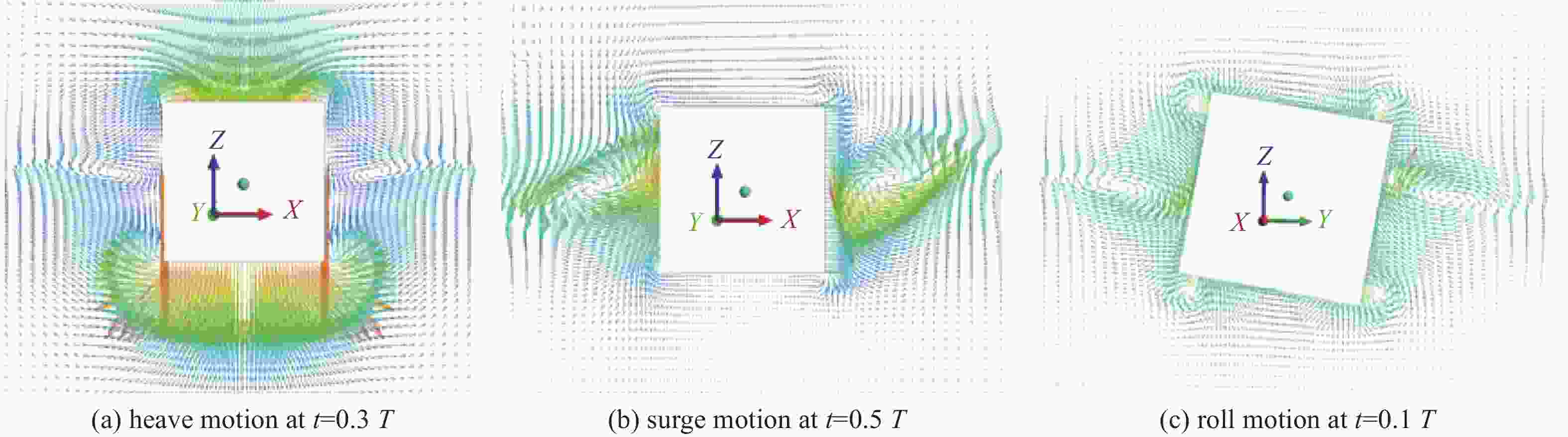
Figure 15.  Velocity vector graphs of flow field for a cube heaving, surging, or rolling in calm water

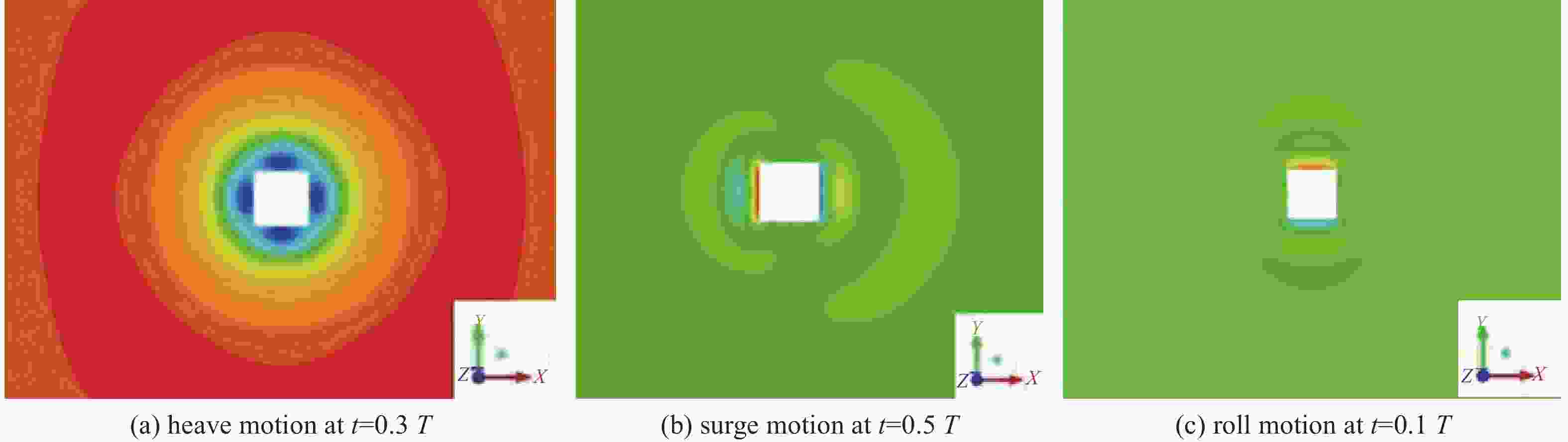
Figure 16.  Contour graphs of free surface for a cube heaving, surging, or rolling in calm water

In this research, a numerical method is proposed to study the hydrodynamic coefficients critical for the design of ocean floating structures, providing fundamental insights into the added mass and damping properties of the structure. The accuracy of the solutions obtained through this computational fluid dynamics (CFD) method is validated by comparison with results derived from potential flow theory. Notably, a high degree of correlation is observed for the heave and surge responses of models at a free surface. For roll, the results are highly sensitive to the mesh applied due to the vortex shedding that occurs at sharp corners, even at relatively low roll amplitudes. This CFD method can be used effectively to study hydrodynamic coefficients of ocean floating structures in a variety of motion modes. By using the current CFD solutions, the added mass, damping coefficients, vector graph of flow field, together with the contour graph of the free surface are also investigated. The most important advantage of this computational method is that the velocity and pressure fields are recorded and visualized by a computer graphics technique at each instant. This is almost impossible experimentally, given the problems of unsteady motion.

The potential flow method is widely used in engineering practice because of its efficiency and accuracy. However, with the improvement of modern engineering requirements, the potential flow method cannot deal with some problems well. In this paper, the two key influencing factors of additional mass and additional damping in the hydrodynamic performance of marine floating structures are analyzed. The additional mass and damping coefficient of marine structures is evaluated more accurately by the proposed viscous flow numerical calculation method. Compared with the potential flow theory, this method can effectively record the pressure field, velocity field and other information, further optimize the stability and performance of the structure, and provide more accurate motion response prediction, which has certain significance for guiding practical engineering.