• Peer Review
  • Non-profit
  • Global Open Access
  • Green Channel for Rising Stars
Volume 11 Issue 1
Jan.  2024
Turn off MathJax
Article Contents

LI Hua. Comparison of wind power density calculation methods based on Weibull distribution [J]. Southern energy construction, 2024, 11(1): 33-41. DOI: 10.16516/j.ceec.2024.1.04 doi:  10.16516/j.ceec.2024.1.04
Citation: LI Hua. Comparison of wind power density calculation methods based on Weibull distribution [J]. Southern energy construction, 2024, 11(1): 33-41. DOI: 10.16516/j.ceec.2024.1.04 doi:  10.16516/j.ceec.2024.1.04

Comparison of Wind Power Density Calculation Methods Based on Weibull Distribution

doi: 10.16516/j.ceec.2024.1.04
  • Received Date: 2023-04-04
  • Rev Recd Date: 2023-06-09
  • Available Online: 2023-09-07
  • Publish Date: 2024-01-10
  •   Introduction  Wind power density is an important parameter for wind resource assessment, and the accurate calculation of wind power density relies on the accuracy of fitting the wind frequency with the Weibull distribution. It is helpful that reasonable analysis the wind power density in that decreasing the risks and improving the decision-making of wind farm investment. Considering the lack of research on the accuracy of Weibull distribution fitting in wind resource assessment, the paper aims to improve the accuracy of wind resource assessment by comparing and studying which method provides a higher accuracy in Weibull distribution fitting.   Method  Five commonly used methods for simulating wind frequency distribution based on the Weibull model were studied. The coefficient of determination was introduced to determine the accuracy of Weibull simulation. The absolute error and relative error between the wind power density calculated by the Weibull function and the wind power density calculated from measured data were compared.   Result  The results show that the energy pattern factor (EPF) method and the maximum likelihood estimation (MLE) method obtained higher coefficients of determination for Weibull fitting compared to other methods, including empirical methods (EPJ and EPL) and the least squares (LLSA) method. The wind power density calculate using these two methods, based on the obtained parameters, has smaller absolute errors and relative errors compared to the other three methods when compared to the wind power density calculate from measured data.   Conclusion  The research results can provide a reference for selecting the appropriate Weibull method to calculate wind power density in wind resource assessment and the true features of wind farm can be revealed, then, the accuracy of wind resource assessment can be improved.
  • [1] 张智伟, 张建平, 刘明, 等. 芦潮港海上风资源变化特性分析 [J]. 发电技术, 2022, 43(2): 260-267. DOI:  10.12096/j.2096-4528.pgt.22010.

    ZHANG Z W, ZHANG J P, LIU M, et al. Analysis on variation characteristics of offshore wind resources in Luchao port [J]. Power generation technology, 2022, 43(2): 260-267. DOI:  10.12096/j.2096-4528.pgt.22010.
    [2] 王稳稳, 胡仁祥, 马瑞, 等. 吐鲁番地区典型风能特性分析 [J]. 内蒙古电力技术, 2022, 40(6): 17-23. DOI:  10.19929/j.cnki.nmgdljs.2022.0092.

    WANG W W, HU R X, MA R, et al. Analysis of typical wind energy characteristics in Turpan [J]. Inner Mongolia electric power, 2022, 40(6): 17-23. DOI:  10.19929/j.cnki.nmgdljs.2022.0092.
    [3] 刘鹏, 王伟胜. 风速概率分布参数的矩估计解法 [J]. 华北电力大学学报, 2002, 29(增刊1): 154-157. DOI:  10.3969/j.issn.1007-2691.2002.z1.037.

    LIU P, WANG W S. The parameter calculation of wind speed probability distribution based on the moment method [J]. Journal of North China Electric Power University, 2002, 29(Suppl. 1): 154-157. DOI:  10.3969/j.issn.1007-2691.2002.z1.037.
    [4] JUSTUS C G, HARGRAVES W R, MIKHAIL A, et al. Methods for estimating wind speed frequency distributions [J]. Journal of applied meteorology and climatology, 1978, 17(3): 350-353. DOI:  10.1175/1520-0450(1978)0172.0.CO;2.
    [5] AKDAĞ S A, DINLER A. A new method to estimate Weibull parameters for wind energy applications [J]. Energy conversion and management, 2009, 50(7): 1761-1766. DOI:  10.1016/j.enconman.2009.03.020.
    [6] STEVENS M J M, SMULDERS P T. The estimation of the parameters of the Weibull wind speed distribution for wind energy utilization purposes [J]. Wind engineering, 1979, 3(2): 132-145.
    [7] STIGLER S M. The history of statistics [M]. Cambridge: Belknap Press of Harvard University Press, 1986.
    [8] 蔡彦枫, 王海龙, 周川, 等. 基于长期实测资料的风速测量相关推测方法对比 [J]. 南方能源建设, 2017, 4(3): 97-102,106. DOI:  10.16516/j.gedi.issn2095-8676.2017.03.018.

    CAI Y F, WANG H L, ZHOU C, et al. Comparison of measure-correlation-predict algorithms in offshore wind power assessment with multi-year observation of automatic weather stations [J]. Southern energy construction, 2017, 4(3): 97-102,106. DOI:  10.16516/j.gedi.issn2095-8676.2017.03.018.
    [9] 肖帆. 基于威布尔分布的风电场风能资源评估及风机选择 [J]. 西北水电, 2017(4): 33-36. DOI:  10.3969/j.issn.1006-2610.2017.04.009.

    XIAO F. Wind energy resources assessment and WTG selection based on Weibull distribution [J]. Northwest hydropower, 2017(4): 33-36. DOI:  10.3969/j.issn.1006-2610.2017.04.009.
    [10] MOHAMMADI K, MOSTAFAEIPOUR A. Using different methods for comprehensive study of wind turbine utilization in Zarrineh, Iran [J]. Energy conversion and management, 2013, 65: 463-470. DOI:  10.1016/j.enconman.2012.09.004.
    [11] TIZPAR A, SATKIN M, ROSHAN M B, et al. Wind resource assessment and wind power potential of Mil-E Nader region in Sistan and Baluchestan Province, Iran – Part 1: annual energy estimation [J]. Energy conversion and management, 2014, 79: 273-280. DOI:  10.1016/j.enconman.2013.10.004.
    [12] BOUDIA S M, GUERRI O. Investigation of wind power potential at Oran, northwest of Algeria [J]. Energy conversion and management, 2015, 105: 81-92. DOI:  10.1016/j.enconman.2015.07.055.
    [13] 李慧, 孙宏斌, 张芳. 风电场风速分布模型研究综述 [J]. 电工电能新技术, 2014, 33(8): 62-66. DOI:  10.3969/j.issn.1003-3076.2014.08.012.

    LI H, SUN H B, ZHANG F. Review on models of wind speed distribution in wind farms [J]. Advanced technology of electrical engineering and energy, 2014, 33(8): 62-66. DOI:  10.3969/j.issn.1003-3076.2014.08.012.
    [14] 龚伟俊, 李为相, 张广明. 基于威布尔分布的风速概率分布参数估计方法 [J]. 可再生能源, 2011, 29(6): 20-23. DOI:  10.13941/j.cnki.21-1469/tk.2011.06.026.

    GONG W J, LI W X, ZHANG G M. The estimation algorithm on the probabilistic distribution parameters of wind speed based on Weibull distribution [J]. Renewable energy resources, 2011, 29(6): 20-23. DOI:  10.13941/j.cnki.21-1469/tk.2011.06.026.
    [15] LYSEN E H. Introduction to wind energy (2nd ed. ) [M]. Amersfoort: SWD Publication, 1983.
    [16] 陈练, 李栋梁, 吴洪宝. 中国风速概率分布及在风能评估中的应用 [J]. 太阳能学报, 2010, 31(9): 1209-1214. DOI:  10.19912/j.0254-0096.2010.09.024.

    CHEN L, LI D L, WU H B. The probability distrubution of wind speed and its application in estimation of wind energy in China [J]. Acta energiae solaris sinica, 2010, 31(9): 1209-1214. DOI:  10.19912/j.0254-0096.2010.09.024.
    [17] COSTA ROCHA P A, DE SOUSA R C, DE ANDRADE C F, et al. Comparison of seven numerical methods for determining Weibull parameters for wind energy generation in the northeast region of Brazil [J]. Applied energy, 2012, 89(1): 395-400. DOI:  10.1016/j.apenergy.2011.08.003.
    [18] SHU Z R, LI Q S, CHAN P W. Statistical analysis of wind characteristics and wind energy potential in Hong Kong [J]. Energy conversion and management, 2015, 101: 644-657. doi:  10.1016/j.enconman.2015.05.070
    [19] 牛鸿燕. 基于Excel规划求解器的配煤比优化尝试 [J]. 科技视界, 2013(12): 130-131. DOI:  10.19694/j.cnki.issn2095-2457.2013.12.100.

    NIU H Y. The optimization of ration coal basis on Excel solver [J]. Science & technology vision, 2013(12): 130-131. DOI:  10.19694/j.cnki.issn2095-2457.2013.12.100.
    [20] 丁思统. 威布尔(Weibull)分布及其拟合 [J]. 江西农业大学学报, 1985(3): 45-52. DOI:  10.13836/j.jjau.1985039.

    DING S T. The Weibull distribution and fitting [J]. Acta Agriculture Universitatis Jiangxiensis, 1985(3): 45-52. DOI:  10.13836/j.jjau.1985039.
    [21] 张雪芝, 王维庆, 王海云. 风电场的风资源评估及产能预估 [J]. 可再生能源, 2017, 35(12): 1876-1880. DOI:  10.13941/j.cnki.21-1469/tk.2017.12.021.

    ZHANG X Z, WANG W Q, WANG H Y. Wind resource assessment and capacity estimation of wind farm [J]. Renewable energy resources, 2017, 35(12): 1876-1880. DOI:  10.13941/j.cnki.21-1469/tk.2017.12.021.
    [22] 袁红亮, 王炎, 陈彬, 等. Meteodyn WT软件的大气热稳定度影响研究 [J]. 西北水电, 2022(3): 113-116. DOI:  10.3969/j.issn.1006-2610.2022.03.022.

    YUAN H L, WANG Y, CHEN B, et al. Study on the influence of atmospheric thermal stability in Meteodyn WT [J]. Northwest hydropower, 2022(3): 113-116. DOI:  10.3969/j.issn.1006-2610.2022.03.022.
  • 通讯作者: 陈斌, bchen63@163.com
    • 1. 

      沈阳化工大学材料科学与工程学院 沈阳 110142

    1. 本站搜索
    2. 百度学术搜索
    3. 万方数据库搜索
    4. CNKI搜索

Figures(5)  / Tables(5)

Article Metrics

Article views(310) PDF downloads(205) Cited by()

Related

Comparison of Wind Power Density Calculation Methods Based on Weibull Distribution

doi: 10.16516/j.ceec.2024.1.04

Abstract:   Introduction  Wind power density is an important parameter for wind resource assessment, and the accurate calculation of wind power density relies on the accuracy of fitting the wind frequency with the Weibull distribution. It is helpful that reasonable analysis the wind power density in that decreasing the risks and improving the decision-making of wind farm investment. Considering the lack of research on the accuracy of Weibull distribution fitting in wind resource assessment, the paper aims to improve the accuracy of wind resource assessment by comparing and studying which method provides a higher accuracy in Weibull distribution fitting.   Method  Five commonly used methods for simulating wind frequency distribution based on the Weibull model were studied. The coefficient of determination was introduced to determine the accuracy of Weibull simulation. The absolute error and relative error between the wind power density calculated by the Weibull function and the wind power density calculated from measured data were compared.   Result  The results show that the energy pattern factor (EPF) method and the maximum likelihood estimation (MLE) method obtained higher coefficients of determination for Weibull fitting compared to other methods, including empirical methods (EPJ and EPL) and the least squares (LLSA) method. The wind power density calculate using these two methods, based on the obtained parameters, has smaller absolute errors and relative errors compared to the other three methods when compared to the wind power density calculate from measured data.   Conclusion  The research results can provide a reference for selecting the appropriate Weibull method to calculate wind power density in wind resource assessment and the true features of wind farm can be revealed, then, the accuracy of wind resource assessment can be improved.

LI Hua. Comparison of wind power density calculation methods based on Weibull distribution [J]. Southern energy construction, 2024, 11(1): 33-41. DOI: 10.16516/j.ceec.2024.1.04 doi:  10.16516/j.ceec.2024.1.04
Citation: LI Hua. Comparison of wind power density calculation methods based on Weibull distribution [J]. Southern energy construction, 2024, 11(1): 33-41. DOI: 10.16516/j.ceec.2024.1.04 doi:  10.16516/j.ceec.2024.1.04
    • 风资源评估是风电开发的重要环节[1],风功率密度又是风能资源评估的重要参数之一[2],是决定风电场是否具有开发潜能的重要评判标准。在年平均风速和空气密度相同的情况下,不同的风频分布将计算得出不同的风功率密度,因而准确分析风资源的风频分布具有重要意义。

      目前,对风频分布的研究多采用威布尔分布,它能比较好地拟合风资源的实际情况。刘鹏等[3]采用了矩估计法模拟风频威布尔分布,此方法简单方便,缺点是不能完全利用风数据样本信息,模拟精度不高。Justus和Lysen提出的经验计算方法[4],被2002版《全国风能评价技术规定》采纳,因简单、实用、耗时短,在风电场建设初期做初步评估时被广泛采用。Akdag 和Dinler提出了用能量因子法来模拟威布尔分布参数[5],此方法目前被广泛应用于风资源流体力学评估模型软件中,如Meteodyn Universe。Stevens MJM 将最大似然法运用于风资源风频分布的模拟计算,并以此估算风电场发电量[6]。最小二乘法由法国勒让德创立,是处理实测值的纯粹代数方法,此方法被广泛应用于各行业,这是一种寻找最佳解,揭示最接近真实情形的状态[7]

      估算风功率密度的方法较多,准确地计算风功率密度有赖于风频威布尔分布拟合的准确性[8]。但是,目前还缺少基于威布尔分布拟合准确性计算风功率密度方面的研究。因此,文章对目前国际常用的5种风频威布尔拟合方法进行对比研究,采用决定系数对威布尔拟合结果准确度进行评价,并在此基础上利用威布尔分布计算风功率密度,并与实测风数据计算所得风功率密度相比较绝对误差和相对误差,从而确定哪些方法更可靠,更准确。文章选取我国不同经纬度和地形地貌的4座测风塔实测数据进行威布尔分布拟合和决定系数分析,并计算相应的风功率密度,用案例进行对比验证得出较优方法,可为工程师在实际的风资源评估工作中提供参考和指导。

    • 威布尔分布是由瑞典科学家威布尔从材料强度的统计理论中推导出来的,是日常生活中一种常用的分布,在风电领域的风频分布中也被广泛采纳应用。

      威布尔的形状参数$k$值反映了风速分布的范围宽窄,一般情况下,$k$值越小,风速分布越宽。当$0 < k < 1$时,风频随着风速的增大而减小,在现实情况中出现较少;当$k = 1$时,风频为指数分布;当$k = 2$时,为瑞利分布;当$k = 3.5$时,接近正态分布。威布尔分布累计概率密度函数如式(1)所示:

      $$ {F_{(v)}} = 1 - {\rm{EXP}}\left[ { - {\left( {\dfrac{v}{c}} \right)^k}} \right] $$ (1)

      式中:

      ${F_{(v)}}$——威布尔风频累计概率密度(%);

      $v$ ——风速(m/s);

      $c$ ——威布尔尺度参数(m/s);

      $k$ ——为威布尔形状参数。

      对威布尔累计概率密度函数(1)求导数,得到威布尔风频分布概率密度函数,如式(2)所示:

      $$ {f_{(v)}} = \dfrac{k}{c}{\left( {\dfrac{v}{c}} \right)^{(k - 1)}}{\rm{EXP}}\left[ { - {\left( {\frac{v}{c}} \right)^k}} \right] $$ (2)

      式中:

      ${f_{(v)}}$——威布尔风频分布概率密度(%)。

      风功率密度是指空气流垂直通过单位截面积的风能,是表征1个地方风能资源多少的1个指标,在风资源评估中一般指年均风功率密度,某地的风功率密度越大,说明该地区风能资源越好[9]。风功率密度计算方法有两种,一种是基于时间序列实测风数据[10],风功率密度与风速的3次方成正比,其计算公式如式(3)所示:

      $$ \overline P = \dfrac{1}{{2n}}\rho \displaystyle \sum\limits_{i = 1}^n {{v_i}^3} = \dfrac{1}{2}\rho \overline {{v_i}^3} $$ (3)

      式中:

      $\overline P $——年均风功率密度(W/m2);

      $\rho $——空气密度(kg/m3);

      ${v_i}$——风速时间序列值(m/s);

      $n$——时间序列。

      另一种是选择合适风速分布的数学模型来模拟风速变化,常见的有双参数威布尔分布、瑞利分布、伽马分布、对数正态分布,大多学者认为双参数威布尔分布可以较好的模拟风速变化[11-13]。基于威布尔分布的风功率密度计算公式如式(4)所示:

      $$ \overline P = \dfrac{1}{2}\rho \int_0^n {{v^3}{f_{(v)}}} {\rm{d}}v $$ (4)
    • 该经验方法由Justus提出[5],我国颁布的《全国风能评价技术规定》中也采用此种方法,此方法计算简单。其$k$值和$c$值计算公式如式(5)和(6)[14]所示:

      $$ k = {\left( {\dfrac{\sigma }{{\overline {{v_i}} }}} \right)^{ - 1.086}} $$ (5)
      $$ c = \dfrac{{\overline {{v_i}} }}{{\Gamma (1 + 1/k)}} $$ (6)

      式中:

      $\sigma $ ——风速标准差(m/s);

      $ \Gamma (1+1/k) $——伽马函数;

      $\overline {{v_i}} $ ——风速序列平均值(m/s)。

    • 此方法由Lysen提出[15],在Justus提出的方法上有所改进,其$k$值计算由式(5)给出,$c$值计算公式如式(7)所示:

      $$ c={\overline{{v}_i}}(0.568+0.433 / k)^{-\tfrac{1}{k}} $$ (7)
    • 基于能量守恒规律,使其威布尔拟合计算得到的风功率密度与实测数据计算所得的风功率密度差值尽可能小的情况下求$k$和$c$值。此方法首先求出能量因子${E_{{\rm{pf}}}}$,其计算公式如式(8)所示,再计算$k$值[16],$k$值计算公式如式(9)所示,$c$值计算公式同式(7):

      $$ {E_{{\rm{pf}}}} = \dfrac{{\dfrac{1}{n}\displaystyle \sum\limits_{i = 1}^n {v_i^3} }}{{{{\left( {\dfrac{1}{n}\displaystyle \sum \limits_{i = 1}^n {v_i}} \right)}^3}}} = \dfrac{{\overline {({v_i}^3)} }}{{{{(\overline {{v_i}} )}^3}}} = \dfrac{{\Gamma (1 + 3/k)}}{{{\Gamma ^3}(1 + 1/k)}} $$ (8)
      $$ k = 1 + \dfrac{{3.69}}{{{{({E_{{\rm{pf}}}})}^2}}} $$ (9)

      式中:

      ${E_{{\rm{pf}}}}$——风功率密度能量因子(W/m2)。

    • 1821年由德国数学家高斯提出最大似然法,此方法首次用于计算发电量可以追溯到Stevens MJM [6],用这种模型来估算风频分布参数$k$和$c$值,其中蕴含的规则是:在求得的$k$和$c$这个特定的威布尔分布函数中,能得到现在的实测风数据序列样本概率最大。

      假设某一风速时间序列样本为:

      $$ V = ({v_1},{v_2},{v_3}...{v_n}) $$

      威布尔概率密度似然函数$f$在某一风速${v_i}$下的公式如式(10)所示:

      $$ {f_{({v_i}\left| {k,c} \right.)}} = \dfrac{k}{c}{\left( {\dfrac{{{v_i}}}{c}} \right)^{(k - 1)}}{\rm{EXP}}\left[ { - {\left( {\dfrac{{{v_i}}}{c}} \right)^k}} \right] $$ (10)

      则风速时间序列样本$V$产生的联合密度函数为:

      $$ \begin{split} &f({v}_{i}|k,c)=f({v}_{1},{v}_{2},{v}_{3},\cdots,{v}_{n}|k,c) =\\&f({v}_{1}|k,c)\times f({v}_{2}|k,c) \times f({v}_{3}|k,c)\times \cdots\times\\& f({v}_{n}|k,c) ={\displaystyle \prod _{i=1}^{n}f({v}_{i}}|k,c)\end{split} $$ (11)

      为了计算方便,等式两边取对数:

      $$ \begin{split} &\ln [f({v_i}\left| {k,c)] = \ln } \right.[\prod\limits_{i = 1}^n {f({v_i}\left| {k,c)} \right.} ] =\\& \ln [f({v_1}\left| {k,c)]} \right. + \ln [f({v_2}\left| {k,c} \right.)] +\\& \ln [f({v_3}\left| {k,c} \right.)] + ...... + \ln [f({v_n}\left| {k,c} \right.)] \\ \end{split} $$ (12)

      上述方程分别对$k$,$c$求导,并令其分别为0,见式(13)和式(15),即可求得威布尔分布的参数$k$和$c$[17],具体见式(14)和式(16):

      $$ \dfrac{{\rm{d}}}{{\rm{d}}k}\mathrm{ln}[f(v|k,c)]=0 $$ (13)
      $$ k = {\left[ {\dfrac{{\displaystyle \sum\nolimits_{i = 1}^n {v_i^k\ln ({v_i})} }}{{\sum\limits_{i = 1}^n {v_i^k} }} - \dfrac{{\displaystyle \sum\limits_{i = 1}^n {\ln ({v_i})} }}{n}} \right]^{ - 1}} $$ (14)
      $$ \dfrac{{\rm{d}}}{{{\rm{d}}c}}\ln [f(v\left| {k,c} \right.)] = 0 $$ (15)
      $$ c = {\left[ {\dfrac{1}{n}\displaystyle \sum\limits_{i = 1}^n {{v_i}^k} } \right]^{1/k}} $$ (16)
    • 风速时间序列某一风速的累计概率密度分布函数公式如式(17)所示:

      $$ F({v_i}) = 1 - {\rm{EXP}}\left[ { - {\left( {\dfrac{{{v_i}}}{c}} \right)^k}} \right] \Rightarrow \frac{1}{1-F\left( {{v}_{i}} \right)}={\rm{EXP}}{\left( {\dfrac{{v}_{i}}{c}} \right)}^{k} $$ (17)

      为计算方便,等式两边取对数如式(18)所示:

      $$ \ln \left[ {\frac{1}{{1 - F({v_i})}}} \right] = {\left( {\frac{{{v_i}}}{c}} \right)^k} \ln [ - \ln (1 - F({v_i})] = k\ln ({v_i}) - k\ln (c) \\ $$ (18)

      累计概率密度函数经过上述的变化推导就变成常见的线性$y = mx + b$形式。最小二乘法的理论基石是实测值与模拟求得的结果值之间的差的平方总和最小。在用于威布尔拟合中,其公式如式(19)所示:

      $$ {\rm{S}}{{\rm{S}}_{{\rm{err}}}} = {\displaystyle \sum\limits_{i = 1}^n {\left( {(k{\text{ln}}({v_i}) - k\ln (c)) - {\text{ln}}\left[ {\dfrac{1}{{1 - F({v_i})}}} \right]} \right)} ^2} $$ (19)

      式中:

      ${\rm{S}}{{\rm{S}}_{{\rm{err}}}}$——为实测值与模拟结果值差的平方总和。

      式(19)对$k$和$c$分别求导,并分别令其为0,得出$k$值和$c$值[18],如式(20)和式(21)所示:

      $$ k = \dfrac{{\displaystyle \sum\limits_{i = 1}^n {[(\ln ({v_i}) - \overline {\ln ({v_i})} ]\left[ {\ln \left( {\dfrac{1}{{1 - F({v_i})}}} \right) - \overline {\ln \left( {\dfrac{1}{{1 - F({v_i})}}} \right)} } \right]} }}{{\displaystyle \sum\limits_{i = 1}^n {[{{(\ln ({v_i}) - \overline {\ln ({v_i})} ]}^2}} }} $$ (20)
      $$ \ln c = \dfrac{{\left( {\overline {\ln \left( {\dfrac{1}{{1 - F({v_i})}}} \right)}} \right) - k\overline {\ln ({v_i})} }}{{ - k}} $$ (21)

      上述最大似然法和最小二乘法所涉及的公式属于理论推导,运算较复杂,在涉及数据繁多的测风数据处理时,常常借助Excel中的规划求解器Slover来解决,Slover规划求解器是一种多次运算组合模拟参数使得目标函数取得最大值或者最小值的解决办法[19],此方法方便快捷,批量处理测风数据能提高计算的效率和准确性。具体运用于此文章时将多次组合模拟$k$和$c$值,使得联合密度函数$ {\displaystyle \prod _{i=1}^{n}f({v}_{i}}|k,c) $取得最大值,最小二乘法函数即式(19)中的${{\rm{SS}}_{{\rm{rr}}}}$取得最小值,此时相应的$k$和$c$即为最优解。

    • 在实际运用中,针对风场实测数据的风频分布情况一般采用上述5种方法进行拟合,文章采用决定系数R2来衡量其拟合结果的精确度[20],其计算公式如式(22)所示:

      $$ {R^2} = 1 - \dfrac{{\displaystyle \sum\nolimits_{i = 1}^n {{{[{f_{\rm{w}}}({v_i}) - {f_{\rm{m}}}({v_i})]}^2}} }}{{\displaystyle \sum\nolimits_{i = 1}^n {{{[{f_{\rm{w}}}({v_i}) - \overline {{f_{\rm{m}}}({v_i})} ]}^2}} }} $$ (22)
      $$ \overline {{f_{\rm{m}}}({v_i})} = \dfrac{1}{{n + 1}}\displaystyle \sum\limits_{i = 1}^n {{f_{\rm{m}}}} ({v_i}) $$ (23)

      式中:

      ${f_{\rm{w}}}({v_i})$——威布尔分布参数计算风速为${v_i}$时的风频(%);

      ${f_{\rm{m}}}({v_i})$——实测风速序列为${v_i}$时的风频(%);

      $\overline {{f_{\rm{m}}}({v_i})}$——实测风速序列风频的平均值(%);

      $ 0.9 < {R^2} \leqslant 1 $,拟合精度好;

      $ 0.8 < {R^2} \leqslant 0.9 $,拟合精度较好;

      $ 0.7 < {R^2} \leqslant 0.8 $,拟合精度一般;

      $ {R^2} \leqslant 0.7 $,拟合精度差。

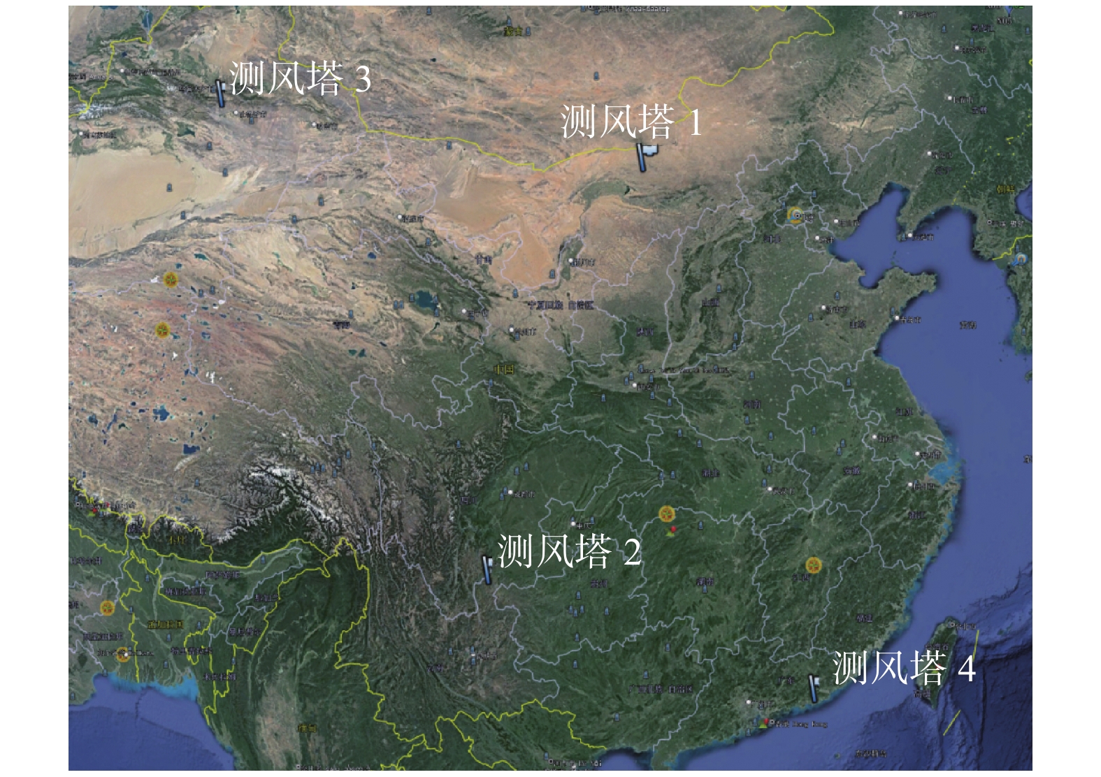
    • 文章选取我国不同经纬度,不同地形地貌及风资源条件各不相同的4座测风塔,1个完整年统计值为10 min的风速样本52560个数据进行分析[21]。测风塔1位于内蒙古茂明的平坦地形,植被稀少地貌非常简单;测风塔2位于云南昭通东部海拔2100 m左右的多山地带,植被较多,地形复杂;测风塔3位于新疆小草湖的半沙漠干旱地带;测风塔4位于广东低纬度甲东地区的沿海滩涂附近。其测风塔所在地理区域位置如图1所示。

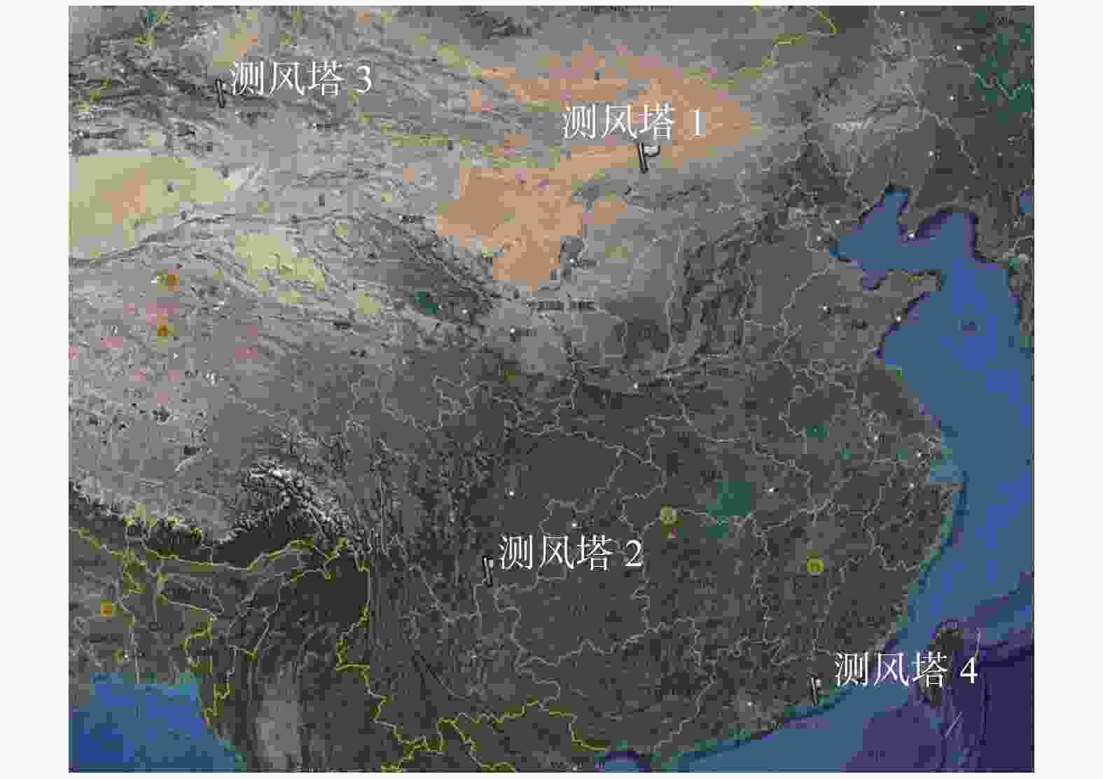
      Figure 1.  The geographic position diagram of 4 masts

      测风塔的经纬度,所在地空气密度,年平均风速和实测风功率密度等基本参数如表1所示。

      测风塔编号经度(E)/(°)纬度(N)/(°)空气密度/(kg·m−3)年均风速/(m·s−1)风速标准差/(m·s−1)最大值/(m·s−1)风功率密度/(W·m−2
      1109.7741.581.127.43.725.3467.50
      2103.6127.350.957.83.127.1426.50
      388.6943.071.109.14.629.5611.90
      4116.1022.811.217.04.124.1521.70

      Table 1.  Wind characteristic parameters

      将测风数据以0.5 m/s作为一个风速区间范围进行频率统计,采用上文介绍的5种威布尔拟合方法分别对收集到的4座测风塔数据进行模拟计算得$k$和$c$值,用威布尔分布函数可以求出各风速段相对应的频率,在此基础上利用式(4)计算威布尔分布风功率密度和式(22)计算决定系数,各测风塔结果分别如表2~表5所示。
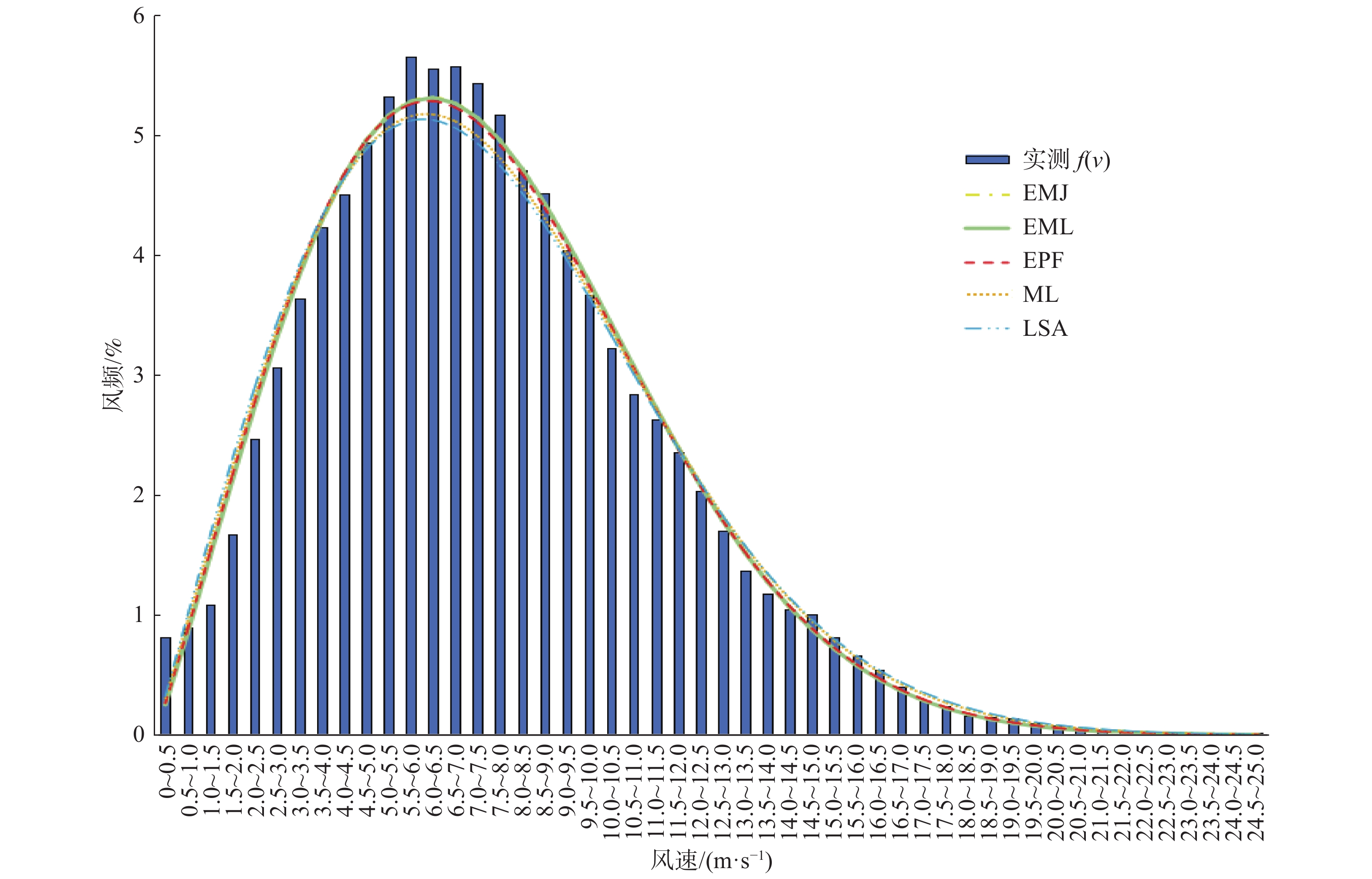
      采用方法经验法EMJ经验法EML能量因子法EPF最大似然法MLE最小二乘法LLSA
      相应参数
      威布尔参数K 2.12 2.12 2.10 2.08 2.03
      威布尔参数C 8.39 8.40 8.40 8.40 8.40
      风功率密度P/(W·m−2 454.20 454.90 457.80 459.50 481.60
      决定系数R2 0.96 0.96 0.97 0.97 0.96

      Table 2.  Simulation results of Weibull distribution and power density of mast 1
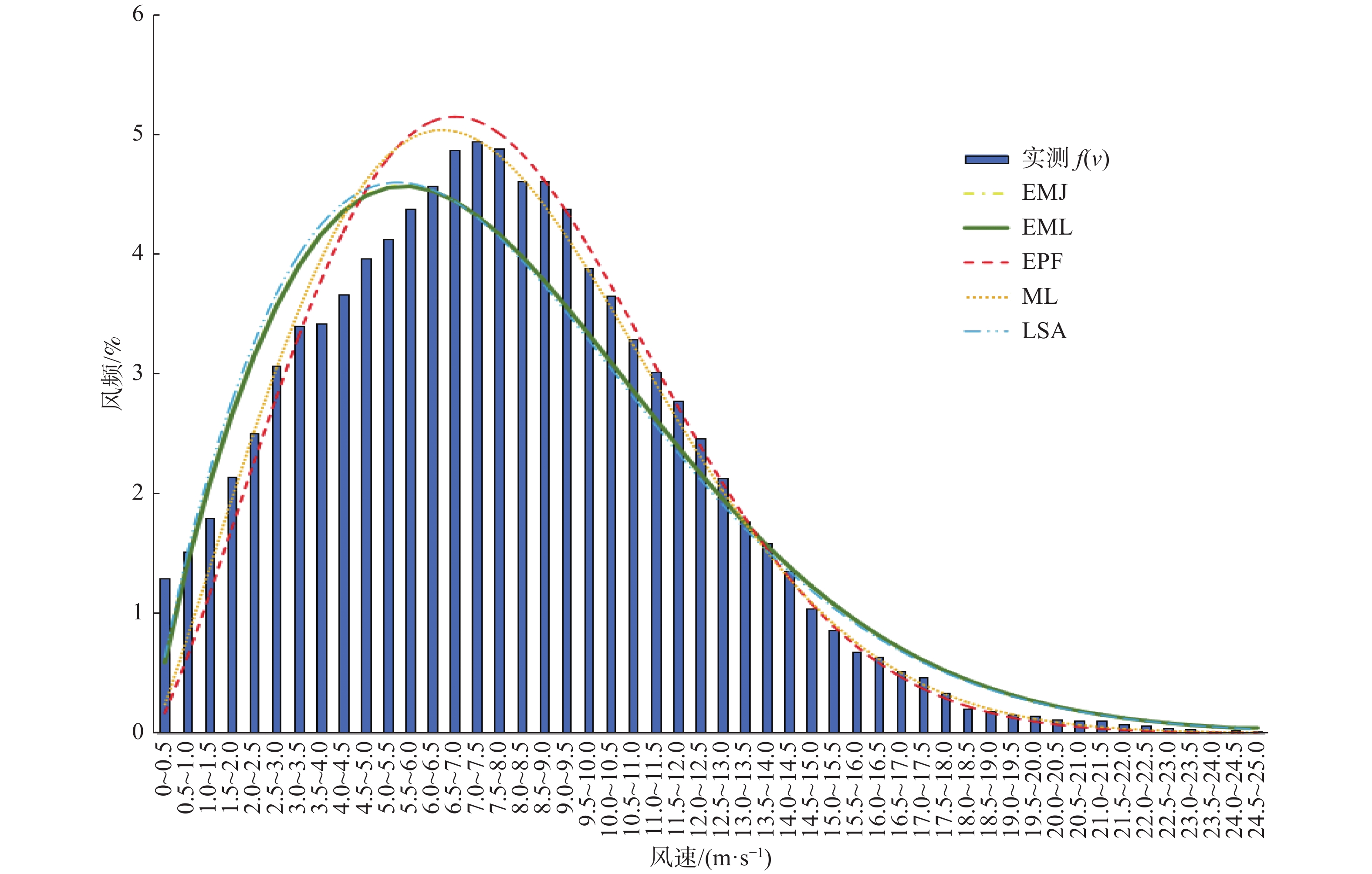
      采用方法经验法EMJ经验法EML能量因子法EPF最大似然法MLE最小二乘法LLSA
      相应参数
      威布尔参数K 1.80 1.80 2.20 2.10 1.78
      威布尔参数C 8.80 8.81 8.90 8.80 8.70
      风功率密度P/(W·m−2 473.46 474.94 405.82 408.64 463.94
      决定系数R2 0.85 0.85 0.92 0.91 0.77

      Table 3.  Simulation results of Weibull distribution and power density of mast 2
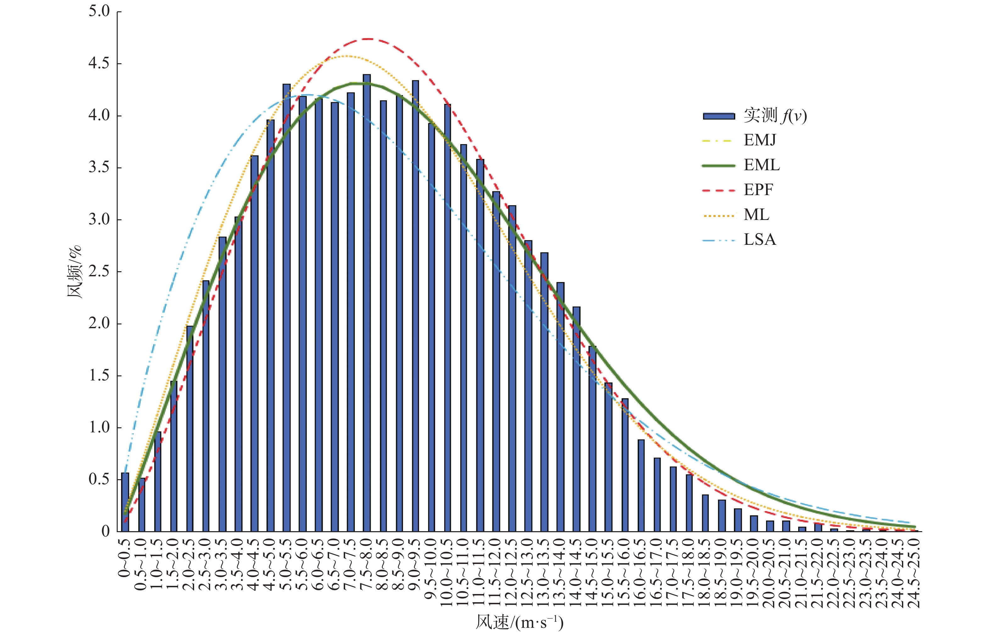
      采用方法经验法
      EMJ
      经验法
      EML
      能量因子法
      EPF
      最大似然法
      MLE
      最小二乘法
      LLSA
      相应参数
      威布尔参数K2.102.102.302.101.77
      威布尔参数C10.2710.2810.009.709.50
      风功率密度
      P/(W·m−2
      737.84739.83640.71628.43680.36
      决定系数R20.690.690.830.850.75

      Table 4.  Simulation results of Weibull distribution and power density of mast 3
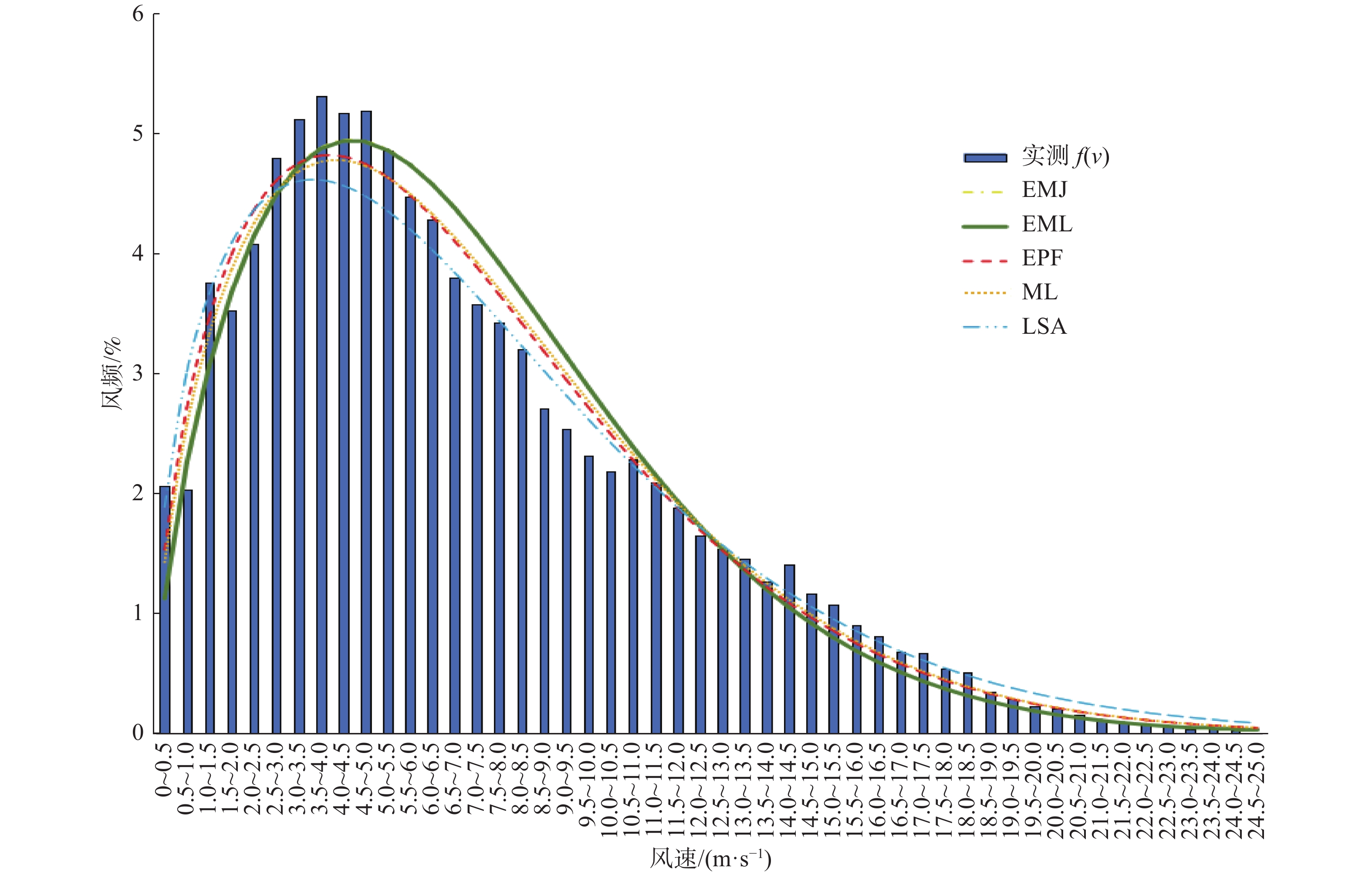
      采用方法经验法EMJ经验法EML能量因子法EPF最大似然法MLE最小二乘法LLSA
      相应参数
      威布尔参数K 1.65 1.65 1.54 1.56 1.45
      威布尔参数C 7.80 7.81 7.80 7.90 8.02
      风功率密度P/(W·m−2 475.58 477.26 515.81 525.36 588.58
      决定系数R2 0.92 0.92 0.96 0.98 0.95

      Table 5.  Simulation results of Weibull distribution and power density of mast 4

      表2~表5模拟结果可知,4座测风塔用经验法EMJ和EML计算的参数值K分别相等,C值均相差0.01,非常接近。

      测风塔1和测风塔4用5种威布尔方法模拟风频结果均好,决定系数均高于0.90,能量因子法EPF和最大似然法MLE的决定系数相对更高,均高于0.96。相应威布尔计算所得的风功率密度与实测数据计算所得风功率密度绝对误差和相对误差也小,其中测风塔1使用能量因子法EPF和最大似然法MLE与实测风数据计算所得风功率467.50 W/m2绝对误差分别为9.70 W/m2和8.00 W/m2,相对误差值分别为2.1%和1.7%。测风塔4用5种威布尔方法计算所得风功率密度和实测风功率密度绝对误差分别为46.12 W/m2,44.44 W/m2,5.89 W/m2,3.66 W/m2和66.88 W/m2

      测风塔2和测风塔3威布尔模拟的决定系数横向比较也有相似的趋势,能量因子法EPF和最大似然法MLE的决定系数高于其他3种方法,其计算所得的风功率密度与实测数据所得风功率密度更加接近,绝对值误差和相对误差均小于其他3种方法。尽管测风塔3模拟决定系数整体偏低,其分布范围为0.69~0.85之间,但能量因子法EPF和最大似然法MLE结果拟合精度较好分别为0.83和0.85,其相对较高的趋势仍未变化。

      测风塔3用能量因子法EPF和最大似然法MLE计算所得的风功率密度与实测数据计算所得风功率密度绝对误差为28.81 W/m2和16.53 W/m2,相对误差分别为4.7%和2.7%;经验法EMJ和EML绝对误差较大,分别为125.94 W/m2和127.93 W/m2,最小二乘法LLSA为68.46 W/m2,相对误差分别为20.6%,17.3%和11.2%。

      测风塔3用经验法EMJ和EML及最小二乘法LLSA威布尔模拟结果一般,决定系数分别为0.69,0.69和0.75,在此基础上利用风频分布计算所得的风功率密度误差更大,这也更好地验证了风频分布拟合准确与否对风功率密度计算准确度影响至关重要,风速与风功率密度是3次方关系。

      4座测风塔实测风频分布图和威布尔分布模拟分布情况如图2~图5所示。

      Figure 2.  Wind speed frequency of the measurement data and Weibull distribution simulation of mast 1

      Figure 3.  Wind speed frequency of the measurement data and Weibull distribution simulation of mast 2

      Figure 4.  Wind speed frequency of the measurement data and Weibull distribution simulation of mast 3

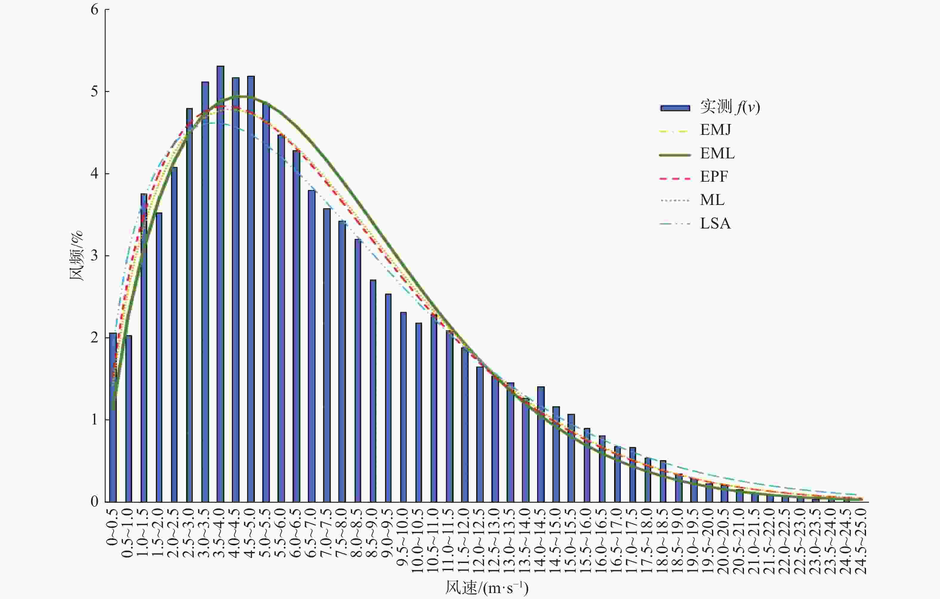
      Figure 5.  Wind speed frequency of the measurement data and Weibull distribution simulation of mast 4

    • 文章针对风频分布拟合方法进行比较研究和风功率密度计算结果验证,引用决定系数对风频分布拟合度进行优劣评价,确定威布尔拟合常用的5种方法准确性高低。为了使结论具有普适性和代表性,文章采用我国不同经纬度,地形地貌各异和风资源禀赋程度各不相同的4座实测测风塔1年统计数据进行验证。

      最终得出结论:威布尔拟合常用的5种计算方法中,能量因子法EPF和最大似然法MLE能更好地拟合实测风数据的风频,采用威布尔计算所得的风功率密度和实测风数据计算的风功率密度更为接近,误差较小,决定系数值较大,其风频的拟合度优于经验法和最小二乘法;经验法和最小二乘法拟合度相对差一些,相应计算的风功率密度误差也大一些。尽管某些测风塔用5种方法拟合所得的决定系数相对都较小,拟合度一般,但横向比较能量因子法EPF和最大似然法MLE的拟合度仍较经验法和最小二乘法有优势,相应计算所得的风功率密度误差仍小于其他3种方法。

      这一结果与目前我国较流行的流体力学风资源模拟软件Meteodyn Universe的运算规则相吻合[22],这款软件在做各高层绘图计算时用的是能量因子法EPF,在各风机机位点参数计算$k$值,$c$值时运用的是最大似然法MLE。

      因此,在实际项目风资源评估中,建议采用能量因子法EPF和最大似然法MLE来模拟风数据的风频分布,计算得出更加接近实际的风功率密度,可为更好地了解掌握风场的风资源提供可靠依据。

Reference (22)

Catalog

    /

    DownLoad:  Full-Size Img  PowerPoint
    Return
    Return