• Peer Review
  • Non-profit
  • Global Open Access
  • Green Channel for Rising Stars
Volume 11 Issue 1
Jan.  2024
Turn off MathJax
Article Contents

LI Sheng, GE Wenpeng, WU Jiacheng, et al. Applicability evaluation of wind turbine wake models [J]. Southern energy construction, 2024, 11(1): 42-53. DOI: 10.16516/j.ceec.2024.1.05 doi:  10.16516/j.ceec.2024.1.05
Citation: LI Sheng, GE Wenpeng, WU Jiacheng, et al. Applicability evaluation of wind turbine wake models [J]. Southern energy construction, 2024, 11(1): 42-53. DOI: 10.16516/j.ceec.2024.1.05 doi:  10.16516/j.ceec.2024.1.05

Applicability Evaluation of Wind Turbine Wake Models

doi: 10.16516/j.ceec.2024.1.05
  • Received Date: 2023-08-01
  • Rev Recd Date: 2023-08-25
  • Available Online: 2023-09-15
  • Publish Date: 2024-01-10
  •   Introduction  The wake effect of wind turbines is an important cause of energy loss in wind farms. The wake study of wind turbines is beneficial to optimization of the turbine arrangement and improvement of the economic efficiency of wind farms.   Method  This paper presented a comparative study of the wake wind speed decay and turbulence intensity prediction of eight common wake models, respectively. To ensure the rationality of the evaluation, the quantitative analysis was carried out based on wind farm measurements and wind tunnel experimental data, and the range of comparison data was limited to 3 to 10 times the diameter downstream the turbine.   Result  The analysis results show that, for the prediction of wake wind speeds, the two-dimensional model fits the actual wake wind speed distribution structure better than the one-dimensional model, in which Jensen-Guass has better wake width prediction ability, while the 2D-k-Jensen wake center wind speed prediction has higher accuracy and adaptability to multiple conditions, with the maximum mean deviation and standard deviation of 8.7% and 5.5%, respectively, which are both applicable to the prediction of turbine wake wind speed. Jensen model has the best prediction ability of wake center wind speed in one-dimensional model, and the mean deviation of some conditions is less than 10%. While Park model is better in predicting the horizontal distribution of wake wind speed. In Case 2, the prediction performance is comparable to that of two-dimensional model, and the mean deviation of each condition is less than 10%, so it is more suitable for wake speed prediction than the former. For the prediction of turbulence intensity, the Ishihara model shows a clear advantage in the prediction of turbulent structure, with mean deviations below 10%, but the prediction of turbulence intensity at the center of the wake is poor, which is not conducive to the prediction of the turbulence intensity at locations downstream the turbine. Among the remaining models, Frandsen and Jensen-Guass models are relatively good at prediction of low ambient turbulence intensities. However, there is an opposite trend between the two for high ambient turbulence intensities: the Frandsen model has higher prediction accuracy and is suitable for turbine turbulence intensity prediction, whereas the prediction result of Jensen-Guass is much larger than the experimental value, and is unstable. The prediction accuracy of wake wind speed for all models is greatly improved at high upstream wind speeds, and the increase in ambient turbulence intensity contributes to the prediction accuracy of the wake wind speed and turbulence intensity for all models, except for the Jensen-Guass model.   Conclusion  The predicted values of wake wind speed for the Jensen-Guass model and the 2D-k-Jensen model coincides better with the measured data, while the prediction performance of the Frandsen model turbulence intensity is better, so they can be used as the reference wake models for the optimization of wind turbine placement and wake control analysis for offshore wind farms.
  • [1] 蔡彦枫, 徐初琪, 汤东升, 等. 基于多尾流模型的大型海上风电场扩容试验研究 [J]. 南方能源建设, 2023, 10(4): 138-147. DOI:  10.16516/j.gedi.issn2095-8676.2023.04.014.

    CAI Y F, XU C Q, TANG D S, et al. Experimental research on capacity expansion of large-scale offshore wind farm under multiple wake models [J]. Southern energy construction, 2023, 10(4): 138-147. DOI:  10.16516/j.gedi.issn2095-8676.2023.04.014.
    [2] 李铮, 郭小江, 申旭辉, 等. 我国海上风电发展关键技术综述 [J]. 发电技术, 2022, 43(2): 186-197. DOI:  10.12096/j.2096-4528.pgt.22028.

    LI Z, GUO X J, SHEN X H, et al. Summary of technologies for the development of offshore wind power industry in China [J]. Power generation technology, 2022, 43(2): 186-197. DOI:  10.12096/j.2096-4528.pgt.22028.
    [3] 宋翌蕾, 田琳琳, 赵宁. 风力机三维尾流模型的提出与校核 [J]. 太阳能学报, 2021, 42(2): 129-135. DOI:  10.19912/j.0254-0096.tynxb.2018-0912.

    SONG Y L, TIAN L L, ZHAO N. Proposal and validation of a new 3D wake model for wind turbine [J]. Acta energiae solaris sinica, 2021, 42(2): 129-135. DOI:  10.19912/j.0254-0096.tynxb.2018-0912.
    [4] JENSEN N O. A note on wind generator interaction [R]. Denmark: Risø National Laboratory, 1983.
    [5] WITHA B, STEINFELD G, HEINEMANN D, et al. Advanced turbine parameterizations in offshore LES wake simulations [C]//Anon. 6. International Symposium on Computational Wind Engineering. Hamburg, Germany, Junelo, 2014. [s. l.]: Witha B, 2014.
    [6] GOIT J P, MEYERS J. Optimal control of energy extraction in wind-farm boundary layers [J]. Journal of fluid mechanics, 2015, 768: 5-50. DOI:  10.1017/jfm.2015.70.
    [7] XIE S B, ARCHER C. Self-similarity and turbulence characteristics of wind turbine wakes via large-eddy simulation [J]. Wind energy, 2015, 18(10): 1815-1838. DOI:  10.1002/we.1792.
    [8] 吴迪, 刘怀西, 苗得胜. 尾流算法与风向变化对海上风机排布影响研究 [J]. 南方能源建设, 2019, 6(2): 54-58. DOI:  10.16516/j.gedi.issn2095-8676.2019.02.010.

    WU D, LIU H X, MIAO D S. Research on offshore wind farm units layout considering the algorithm of wake model and the change of wind direction [J]. Southern energy construction, 2019, 6(2): 54-58. DOI:  10.16516/j.gedi.issn2095-8676.2019.02.010.
    [9] KATIC I, HØJSTRUP J, JENSEN N O. A simple model for cluster efficiency [C]//Anon. European Wind Energy Association Conference and Exhibition, Rome, Italy, October 6-8, 1986. Rome: A. Raguzzi, 1987.
    [10] FRANDSEN S, BARTHELMIE R, PRYOR S, et al. Analytical modelling of wind speed deficit in large offshore wind farms [J]. Wind energy, 2006, 9(1/2): 39-53. DOI:  10.1002/we.189.
    [11] PORTÉ-AGEL F, WU Y T, CHEN C H. A numerical study of the effects of wind direction on turbine wakes and power losses in a large wind farm [J]. Energies, 2013, 6(10): 5297-5313. DOI:  10.3390/en6105297.
    [12] CHAMORRO L P, PORTÉ-AGEL F. Effects of thermal stability and incoming boundary-layer flow characteristics on wind-turbine wakes: a wind-tunnel study [J]. Boundary-layer meteorology, 2010, 136(3): 515-533. DOI:  10.1007/s10546-010-9512-1.
    [13] XIE S B, ARCHER C L. A numerical study of wind-turbine wakes for three atmospheric stability conditions [J]. Boundary-layer meteorology, 2017, 165(1): 87-112. DOI:  10.1007/s10546-017-0259-9.
    [14] LI Q, MURATA J, ENDO M, et al. Experimental and numerical investigation of the effect of turbulent inflow on a horizontal axis wind turbine (part II: wake characteristics) [J]. Energy, 2016, 113: 1304-1315. DOI:  10.1016/j.energy.2016.08.018.
    [15] 杨祥生. 风力机尾流效应数值模拟研究 [D]. 南京: 南京航空航天大学, 2016.

    YANG X S. Study on the numerical simulation of wind turbine wakes effect [D]. Nanjing: Nanjing University of Aeronautics and Astronautics, 2016.
    [16] AINSLIE J F. Calculating the flowfield in the wake of wind turbines [J]. Journal of wind engineering and industrial aerodynamics, 1988, 27(1-3): 213-224. DOI:  10.1016/0167-6105(88)90037-2.
    [17] MAGNUSSON M. Near-wake behaviour of wind turbines [J]. Journal of wind engineering and industrial aerodynamics, 1999, 80(1/2): 147-167. DOI:  10.1016/S0167-6105(98)00125-1.
    [18] CRESPO A, HERNÁNDEZ J. Turbulence characteristics in wind-turbine wakes [J]. Journal of wind engineering and industrial aerodynamics, 1996, 61(1): 71-85. DOI:  10.1016/0167-6105(95)00033-X.
    [19] FRANDSEN S. Measurements on and modelling of offshore wind farms [R]. Denmark: Forskningscenter Risoe, 1996.
    [20] TIAN L L, ZHU W J, SHEN W Z, et al. Development and validation of a new two-dimensional wake model for wind turbine wakes [J]. Journal of wind engineering and industrial aerodynamics, 2015, 137: 90-99. DOI:  10.1016/j.jweia.2014.12.001.
    [21] GAO X X, YANG H X, LU L. Optimization of wind turbine layout position in a wind farm using a newly-developed two-dimensional wake model [J]. Applied energy, 2016, 174: 192-200. DOI:  10.1016/j.apenergy.2016.04.098.
    [22] ISHIHARA T, QIAN G W. A new Gaussian-based analytical wake model for wind turbines considering ambient turbulence intensities and thrust coefficient effects [J]. Journal of wind engineering and industrial aerodynamics, 2018, 177: 275-292. DOI:  10.1016/j.jweia.2018.04.010.
    [23] 吴阳阳. 基于测风数据的经验尾流模型适用性分析研究 [J]. 浙江电力, 2017, 36(11): 92-98. DOI:  10.19585/j.zjdl.201711017.

    WU Y Y. Applicability analysis of empirical wake model based on wind data [J]. Zhejiang electric power, 2017, 36(11): 92-98. DOI:  10.19585/j.zjdl.201711017.
    [24] CAMPAGNOLO F, MOLDER A, SCHREIBER J, et al. Comparison of analytical wake models with wind tunnel data [J]. Journal of physics: conference series, 2019, 1256: 012006. DOI:  10.1088/1742-6596/1256/1/012006.
    [25] BARTHELMIE R J, LARSEN G C, FRANDSEN S T, et al. Comparison of wake model simulations with offshore wind turbine wake profiles measured by sodar [J]. Journal of atmospheric and oceanic technology, 2006, 23(7): 888-901. DOI:  10.1175/JTECH1886.1.
    [26] GӦÇMEN T, LAAN P V D, RÉTHORÉ P E, et al. Wind turbine wake models developed at the technical university of Denmark: a review [J]. Renewable and sustainable energy reviews, 2016, 60: 752-769. DOI:  10.1016/j.rser.2016.01.113.
    [27] JEON S, KIM B, HUH J. Comparison and verification of wake models in an onshore wind farm considering single wake condition of the 2 MW wind turbine [J]. Energy, 2015, 93: 1769-1777. DOI:  10.1016/j.energy.2015.09.086.
  • 通讯作者: 陈斌, bchen63@163.com
    • 1. 

      沈阳化工大学材料科学与工程学院 沈阳 110142

    1. 本站搜索
    2. 百度学术搜索
    3. 万方数据库搜索
    4. CNKI搜索

Figures(17)  / Tables(4)

Article Metrics

Article views(438) PDF downloads(125) Cited by()

Related

Applicability Evaluation of Wind Turbine Wake Models

doi: 10.16516/j.ceec.2024.1.05

Abstract:   Introduction  The wake effect of wind turbines is an important cause of energy loss in wind farms. The wake study of wind turbines is beneficial to optimization of the turbine arrangement and improvement of the economic efficiency of wind farms.   Method  This paper presented a comparative study of the wake wind speed decay and turbulence intensity prediction of eight common wake models, respectively. To ensure the rationality of the evaluation, the quantitative analysis was carried out based on wind farm measurements and wind tunnel experimental data, and the range of comparison data was limited to 3 to 10 times the diameter downstream the turbine.   Result  The analysis results show that, for the prediction of wake wind speeds, the two-dimensional model fits the actual wake wind speed distribution structure better than the one-dimensional model, in which Jensen-Guass has better wake width prediction ability, while the 2D-k-Jensen wake center wind speed prediction has higher accuracy and adaptability to multiple conditions, with the maximum mean deviation and standard deviation of 8.7% and 5.5%, respectively, which are both applicable to the prediction of turbine wake wind speed. Jensen model has the best prediction ability of wake center wind speed in one-dimensional model, and the mean deviation of some conditions is less than 10%. While Park model is better in predicting the horizontal distribution of wake wind speed. In Case 2, the prediction performance is comparable to that of two-dimensional model, and the mean deviation of each condition is less than 10%, so it is more suitable for wake speed prediction than the former. For the prediction of turbulence intensity, the Ishihara model shows a clear advantage in the prediction of turbulent structure, with mean deviations below 10%, but the prediction of turbulence intensity at the center of the wake is poor, which is not conducive to the prediction of the turbulence intensity at locations downstream the turbine. Among the remaining models, Frandsen and Jensen-Guass models are relatively good at prediction of low ambient turbulence intensities. However, there is an opposite trend between the two for high ambient turbulence intensities: the Frandsen model has higher prediction accuracy and is suitable for turbine turbulence intensity prediction, whereas the prediction result of Jensen-Guass is much larger than the experimental value, and is unstable. The prediction accuracy of wake wind speed for all models is greatly improved at high upstream wind speeds, and the increase in ambient turbulence intensity contributes to the prediction accuracy of the wake wind speed and turbulence intensity for all models, except for the Jensen-Guass model.   Conclusion  The predicted values of wake wind speed for the Jensen-Guass model and the 2D-k-Jensen model coincides better with the measured data, while the prediction performance of the Frandsen model turbulence intensity is better, so they can be used as the reference wake models for the optimization of wind turbine placement and wake control analysis for offshore wind farms.

LI Sheng, GE Wenpeng, WU Jiacheng, et al. Applicability evaluation of wind turbine wake models [J]. Southern energy construction, 2024, 11(1): 42-53. DOI: 10.16516/j.ceec.2024.1.05 doi:  10.16516/j.ceec.2024.1.05
Citation: LI Sheng, GE Wenpeng, WU Jiacheng, et al. Applicability evaluation of wind turbine wake models [J]. Southern energy construction, 2024, 11(1): 42-53. DOI: 10.16516/j.ceec.2024.1.05 doi:  10.16516/j.ceec.2024.1.05
    • 由于全球能源储备的紧缺以及化石能源的污染问题,风能等清洁能源规模不断扩大,能源消费占比将逐渐提高,海上风场发展也呈现出大容量、集中化等特点[1-2]。对于规模化海上风场,上游机组所产生的尾流势必会导致下游机组发电量有所下降,强湍流和附加的风剪切会影响下游机组的疲劳载荷、结构性能和使用寿命[3]。因此详细了解机组尾流速度和湍流分布,进而优化设计海上风场机位排布成为当下的热门话题。

      风场机组尾流计算主要有3种方式,基于实验数据拟合的半经验尾流模型[4]、基于势流理论的制动盘或制动线模型[5-6]、基于N-S方程的CFD模型[7]。后两者虽计算结果精度更高,但因其所需的庞大计算资源,无法适应快节奏的风场项目工程需求,使得两者在实际工程中的运用受到极大限制。而半经验尾流模型因具备计算效率高,计算精度满足工程要求等优势而受到WT、WASP等风资源商业软件[8]的青睐,且被广泛应用于风场前期规划设计中。半经验尾流模型最早由Jensen[4]提出,后来由Katic等[9]和Frandsen等[10]进一步开发,该模型结构简单、计算效率高且通过数值实验[11]证明了预测性能,但其帽型的风速分布并不符合实际机组尾流情况[12]。数值模拟[13]和风洞测量[14]均表明,尾流速度剖面近似于高斯曲线,杨祥生[15]基于尾流风速高斯对称分布假设对Park模型[9]进行修正,提出了二维尾流模型。至此以上模型均未考虑湍流的动态影响,但尾流湍流特性的分析式早在1988年便已出现,例如Ainslie等[16]、Magnusso等[17]、Crespo等[18]、Frandsen等[19],因此一些学者在尾流风速预估中进一步考虑了尾流湍流的影响[20-21]。Ishihara等[22]考虑高度方向的风速变化,进一步提出了三维尾流模型。对于尾流模型适用性研究方面,吴阳阳[23]仅通过一组风洞实验数据研究了3种一维模型的优缺点,Campagnolo等[24]所研究的尾流模型参数均根据两组实验工况进行定制化寻优,无法较好得到模型多工况下适用性情况。

      目前机组半经验尾流模型相关研究大多集中在单一尾流模型的提出和优化上,对于多个尾流模型的全面对比分析相关研究较少。本文对8个常见风力机组尾流模型进行了系统的研究,依托3组风场实测或风洞实验数据,着重分析了各模型尾流风速和湍流强度的预估情况,为海上风场机位排布优化及尾流控制分析的尾流模型选择提供参考。

    • 本文对几个尾流模型的尾流速度和湍流强度预测进行研究,各模型所具备的预测功能如表1所示。

      模型 尾流速度 湍流强度
      Jensen ×
      Park ×
      Frandsen
      Crespo ×
      2D-k-Jensen
      Jensen-Gauss
      Park-Gauss ×
      Ishihara
      注:“√”表明具备该预测功能;“×”表明不具备该预测功能。

      Table 1.  Summary of model prediction functions

    • Jensen[4]尾流模型是一维(1D)尾流模型,利用两个公式来计算尾流半径区域及风速恢复情况,其尾流线性扩展、风速恢复率恒定,轮毂高度处尾流风速水平分布呈“帽形”,如图1所示,图中xy分别为轮毂高度处下游方向和展向距离,经验公式如下:

      Figure 1.  Jensen wake model

      $$ {D}_{{\rm{w}}}=2\times (k\times x+{r}_{0}) $$ (1)
      $$ U={U}_{0}\left[1-\frac{2}{3}\left(\frac{{r}_{0}}{{r}_{0}+k\times x}\right)\right] $$ (2)

      式中:

      $ {D}_{{\rm{w}}} $ ——尾流直径(m);

      $ k $ ——尾流膨胀系数;

      $ x $ ——机组下游距离(m);

      $ {r}_{0} $ ——风力机叶轮半径(m);

      $ U $ ——尾流速度(m/s);

      $ {U}_{0} $ ——环境风速(m/s)。

      其中尾流膨胀系数$ k $随风力机所在地形和气象条件的不同,其取值有所差别,文献[25]建议陆上应用取0.075,海上应用取0.04或0.05,而文献[26]基于相似性理论将尾流膨胀系数与湍流强度相关联,尾流膨胀系数为:

      $$ k \approx 0.4\times I $$ (3)

      式中:

      I——轮毂高度处湍流强度。

    • Katic等[9]在Jensen模型基础上进一步提出了包括实际风机物理特性的1D模型,Katic等人的尾流模型没有使用常见的高斯分布,而是假设尾流区域内的风速恒定。尾流风速计算公式:

      $$ U={{U}_{0}-U}_{0}\times \frac{\left(1-\sqrt{1-{C}_{{\rm{T}}}}\right)}{{\left(1+\dfrac{2\times k\times x}{{D}_{0}}\right)}^{2}} $$ (4)

      式中:

      $ {C}_{{\rm{T}}} $ ——推力系数;

      $ D $ ——风力机叶轮直径(m)。

    • Frandsen等在1996年提出了关于尾流湍流强度预测的经验模型[19],湍流强度值随下游距离恒定变化,并在2006年基于动量守恒方程,提出了Storpark分析模型(SAM)[10],用于计算尾流直径和尾流风速值,SAM也假设了“顶帽”形状的尾流发展,具体公式为:

      $$ {I}_{{\rm{wave}}}=\sqrt{{K}_{{\rm{n}}}\frac{{C}_{{\rm{T}}}}{{s}^{2}}+{{I}_{0}}^{2}} $$ (5)
      $$ U={U}_{0}\left(\frac{1}{2}+\frac{1}{2}\sqrt{1-2\frac{{{D}_{0}}^{2}}{{{D}_{{\rm{w}}}}^{2}}{C}_{{\rm{T}}}}\right) $$ (6)
      $$ \frac{{D}_{{\rm{w}}}}{D}={\left({\beta }^{K/2}+\alpha \times s\right)}^{1/K} $$ (7)
      $$ \alpha ={\beta }^{K/2}\left[{\left(1+2\times {\alpha }_{\left({\rm{noj}}\right)}\times s\right)}^{K}-1\right]{s}^{-1} $$ (8)
      $$ \beta =\frac{1}{2}\frac{1+\sqrt{1-{C}_{{\rm{T}}}}}{\sqrt{1-{C}_{{\rm{T}}}}} $$ (9)
      $$ s=x/D $$ (10)

      式中:

      $ {I}_{{\rm{wave}}} $ ——尾流湍流强度;

      $ {K}_{{\rm{n}}} $ ——模型参数,取0.4;

      $ {I}_{0} $ ——环境湍流强度;

      $ {\alpha }_{\left({\rm{noj}}\right)} $ ——控制尾流恢复的参数,取0.05;

      K ——控制尾流恢复的参数,取3。

    • Crespo和Hernandez[18]在1996年基于实验和数值方法提出了湍流强度预测经验表达式,该模型同样预测出恒定的湍流强度分布,如下:

      $$ {I}_{{\rm{add}}}=0.73\times {a}^{0.832\;5}\times {{I}_{0}}^{0.032\;5}\times {(x/D)}^{-0.32} $$ (11)
      $$ a=\frac{1}{2}-\frac{1}{2}\left(\sqrt{1-{C}_{{\rm{T}}}}\right) $$ (12)
      $$ {I}_{{\rm{wave}}}=\sqrt{{{I}_{0}}^{2}+{{I}_{{\rm{add}}}}^{2}} $$ (13)

      式中:

      $ {I}_{{\rm{add}}} $ ——风力机组产生的附加湍流强度;

      $ a $ ——风力机组轴向诱导因子。

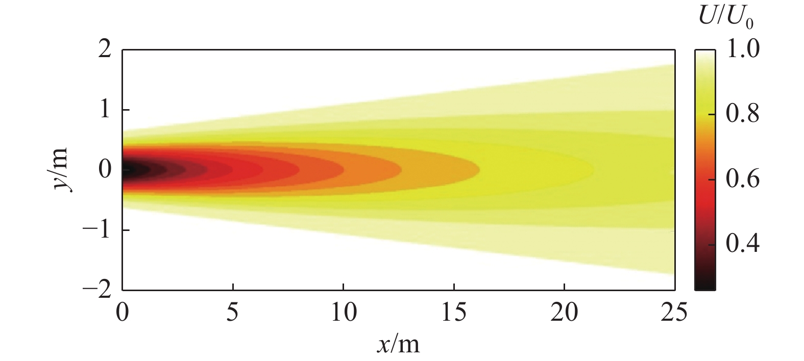
    • Tian等[20]在Jensen模型的基础上,通过引入余弦形而非“顶帽”形的风速分布构建了一种新的二维(2D)尾流横截面风速预测模型,如图2所示,该模型采用一个可变的尾流膨胀系数综合考虑了环境湍流与附加湍流的共同作用,尾流膨胀为非线性状态,其尾流速度与湍流强度计算公式如下:

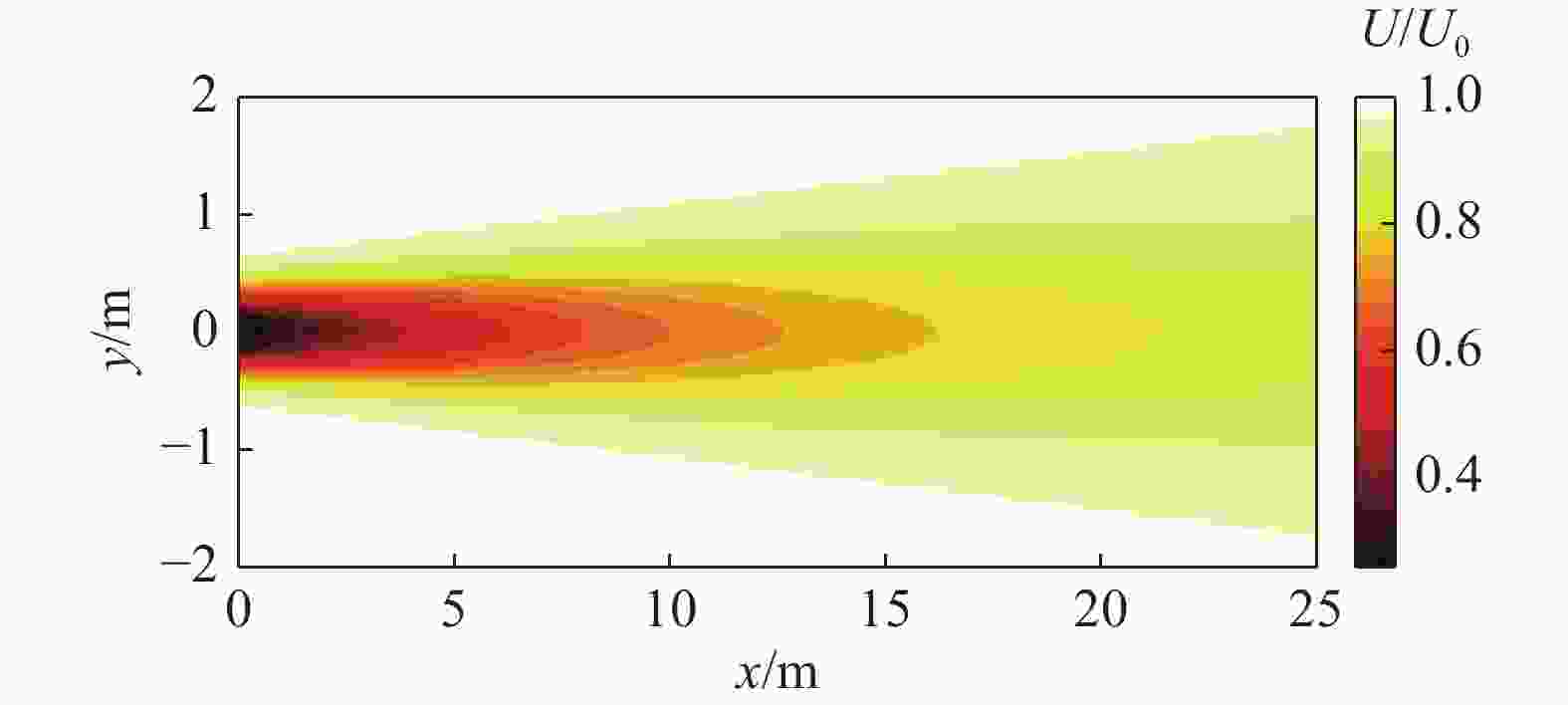
      Figure 2.  2D-k-Jensen wake model

      $$ {I}_{{\rm{wave}}}={K}_{{\rm{n}}}\times \frac{{C}_{{\rm{T}}}}{x/{D}_{0}}+{I}_{0} $$ (14)
      $$ {k}_{{\rm{wave}}}=k\times \frac{{I}_{{\rm{wave}}}}{{I}_{0}} $$ (15)
      $$ {r}_{x}={k}_{{\rm{wave}}}\times x+{r}_{0} $$ (16)
      $$ {r}_{1}={r}_{0}\times \sqrt{\frac{1-a}{1-2a}} $$ (17)
      $$ {U}^{\mathrm{*}}={U}_{0}\left[1-\dfrac{2\times a}{{\left(1+\dfrac{{k}_{{\rm{wave}}}\times x}{{r}_{1}}\right)}^{2}}\right] $$ (18)
      $$ U=\left({U}_{0}-{U}^{\mathrm{*}}\right)\times {\rm{cos}}\left(\frac{{\text{π}} }{{r}_{x}}\times r+{\text{π}} \right)+{U}^{\mathrm{*}} $$ (19)

      式中:

      $ {k}_{{\rm{wave}}} $ ——综合考虑环境湍流和附加湍流后的尾流膨胀系数;

      $ {r}_{x} $ ——下游x距离的尾流半径(m);

      $ {r}_{1} $ ——刚经过风轮后的尾流半径(m);

      $ r $ ——距轮毂中心的Y向距离(m)。

    • 基于Jensen尾流模型和风机尾流柱段的高斯分布理论,Gao等[21]开发了一个二维分析尾流模型。为考虑环境湍流和风力机产生的附加湍流的影响,该模型与2D-k-Jensen模型进行了相似的处理,尾流膨胀系数k用$ {k}_{{\rm{wave}}} $代替,具体公式如下:

      $$ {r}_{x}={k}_{{\rm{wave}}}\times x+{r}_{1} $$ (20)
      $$ {I}_{{\rm{wave}}}={\left[{K}_{{\rm{n}}}\times \frac{{C}_{{\rm{T}}}}{{\left(\dfrac{x}{{D}_{0}}\right)}^{0.5}}+{{I}_{0}}^{0.5}\right]}^{2} $$ (21)
      $$ {U}^{\mathrm{*}}={U}_{0}\left[1-\frac{2\times a}{{\left(1+\dfrac{{k}_{{\rm{wave}}}\times x}{{r}_{1}}\right)}^{2}}\right] $$ (22)
      $$ U={U}_{0}-\left({U}_{0}-{U}^{\mathrm{*}}\right)\times \frac{5.16}{\sqrt{2{\text{π}}}}\times {e}^{\tfrac{-{r}^{2}}{2\times {\left(\tfrac{{r}_{x}}{2.58}\right)}^{2}}} $$ (23)
    • 杨祥生[15]基于Park模型尾流区线性膨胀假设、径向风速呈高斯分布提出了Park-Gauss尾流模型,用于预测风力机尾流速度损失,具体公式如下:

      $$ {r}_{x}=k\times x+{r}_{1} $$ (24)
      $$ {U}^{\mathrm{*}}={U}_{0}\left[1-\frac{2\times a}{{\left(1+\dfrac{k\times x}{{r}_{1}}\right)}^{2}}\right] $$ (25)
      $$ U={U}_{0}+\frac{{U}_{0}-{U}^{\mathrm{*}}}{1-\dfrac{26{\mathrm{e}}}{35}}\times ({{\mathrm{e}}}^{1-{\left(\tfrac{r}{{r}_{x}}\right)}^{2}}-1) $$ (26)
    • Ishihara和Qian[22]通过风力机组尾流大涡模拟数值分析研究,提出了一种新的尾流模型,该模型风速预测假设风机下游区域具有线性尾流衰减、自相似性和高斯轴对称性,湍流强度水平分布预估出双高斯形,计算式如下:

      $$ {k}^{*}=0.11\times {{C}_{{\rm{T}}}}^{1.07}\times {{I}_{0}}^{0.2} $$ (27)
      $$ \varepsilon =0.23\times {{C}_{{\rm{T}}}}^{-0.25}\times {{I}_{0}}^{0.17} $$ (28)
      $$ a=0.93\times {{C}_{{\rm{T}}}}^{-0.75}\times {{I}_{0}}^{0.17} $$ (29)
      $$ b=0.42\times {{C}_{{\rm{T}}}}^{0.6}\times {{I}_{0}}^{0.2} $$ (30)
      $$ c=0.15\times {{C}_{{\rm{T}}}}^{-0.25}\times {{I}_{0}}^{-0.7} $$ (31)
      $$ d=2.3\times {{C}_{{\rm{T}}}}^{-1.2},e=1.0\times {{I}_{0}}^{0.1} $$ (32)
      $$ f=0.7\times {{C}_{{\rm{T}}}}^{-3.2}\times {{I}_{0}}^{-0.45} $$ (33)
      $$ \frac{\sigma }{D}={k}^{*}\times \frac{x}{{D}_{0}}+\varepsilon ,r=\sqrt{{y}^{2}+{(z-H)}^{2}} $$ (34)
      $$ \frac{{U}_{h}-U}{{U}_{h0}}=\dfrac{1}{{[a+b\times \dfrac{x}{{D}_{0}}+c\times {(1+\dfrac{x}{{D}_{0}})}^{-2}]}^{2}}\times \mathrm{e}\mathrm{x}\mathrm{p}\left(-\dfrac{{r}^{2}}{2\times {\sigma }^{2}}\right) $$ (35)
      $$ {k}_{1}=\left\{\begin{array}{l}{{\rm{cos}}}^{2}\left[\dfrac{{\text{π}} }{2}\times \left(\dfrac{r}{{D}_{0}}-0.5\right)\right]\dfrac{r}{{D}_{0}}\leqslant 0.5\\ 1\dfrac{r}{{D}_{0}} > 0.5\end{array}\right. $$ (36)
      $$ {k}_{2}=\left\{\begin{array}{l}{{\rm{cos}}}^{2}\left[\dfrac{{\text{π}}}{2}\times \left(\dfrac{r}{{D}_{0}}+0.5\right)\right]\dfrac{r}{{D}_{0}}\leqslant 0.5\\ 0\dfrac{r}{{D}_{0}} > 0.5\end{array}\right. $$ (37)
      $$ {\delta }_{z}=\left\{\begin{array}{l}{{I}_{0}\times {\rm{sin}}}^{2}\left({\text{π}} \times \dfrac{H-z}{H}\right)z < H\\ 0z\geqslant H\end{array}\right. $$ (38)
      $$ \begin{array}{l} {I_{{\rm{add}}}} = \dfrac{1}{{d + e \times \dfrac{x}{{{D_0}}} + f \times {{\left( {1 + \dfrac{x}{{{D_0}}}} \right)}^{ - 2}}}} \times \\ \left\{ {{k_1} \times {\rm{exp}}\left( { - \dfrac{{{{\left( {r - {r_0}} \right)}^2}}}{{2 \times {\sigma ^2}}}} \right) + {k_2} \times {\rm{exp}}\left( { - \dfrac{{{{\left( {r + {r_0}} \right)}^2}}}{{2 \times {\sigma ^2}}}} \right)} \right\} - {\delta _z} \end{array} $$ (39)
      $$ {I}_{{\rm{wave}}}=\sqrt{{{I}_{0}}^{2}+{{I}_{{\rm{add}}}}^{2}} $$ (40)

      式中:

      $ {U}_{h0} $ ——轮毂高度的平均风速(m/s);

      $ {U}_{h} $ ——某高度位置的环境风速(m/s);

      $ {\textit{z}} $ ——据风机底部垂直方向距离(m);

      $ \sigma $ ——代表性尾流宽度(m);

      $ H $ ——轮毂高度(m);

      $ {k}^{*}、\varepsilon $ ——尾流宽度预测模型参数;

      $ a $、$ b $、$ c $ ——风速预测模型参数;

      $ {k}_{1}\mathrm{、}{k}_{2}\mathrm{、}d $、$ e $、$ f $、$ {\delta }_{z} $ ——湍流强度模型参数。

    • 本文基于风场测量、风洞实验等3个不同的实测数据来论证各尾流模型的预测性能,其中尾流速度的对比分析采用案例1和案例2,湍流强度通过案例2和案例3进行研究。

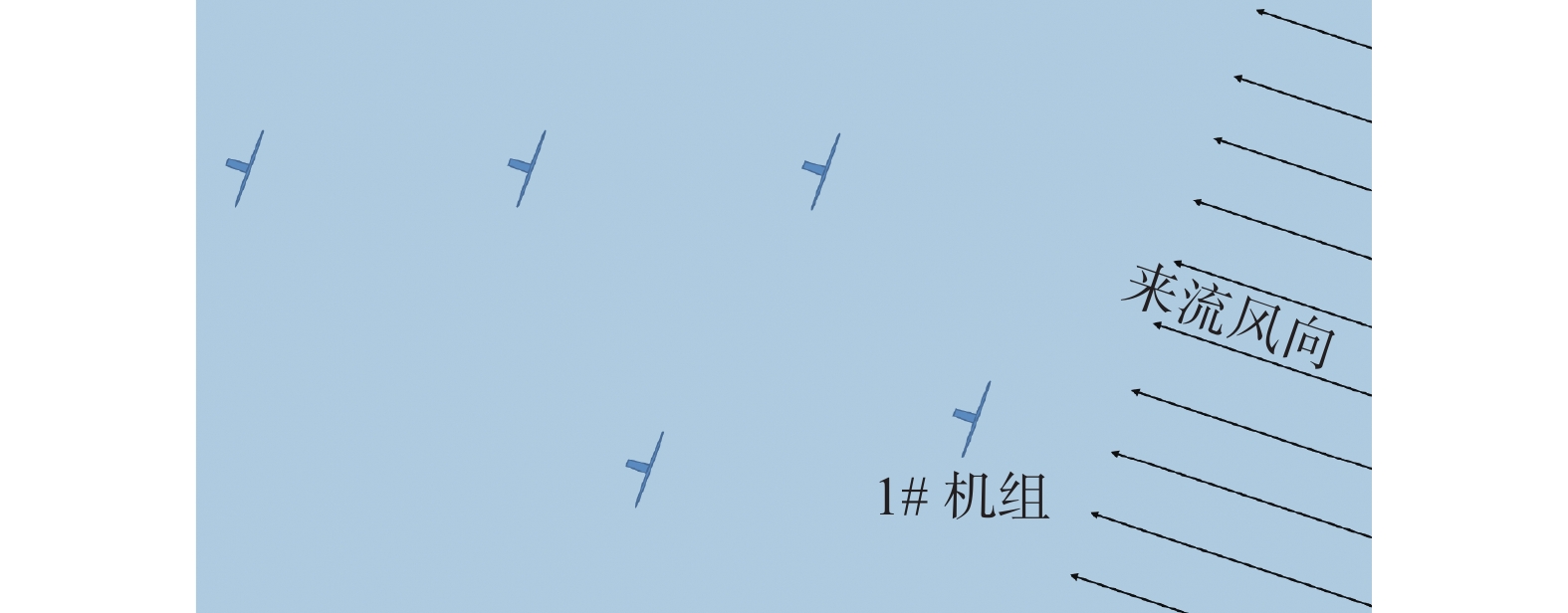
    • 该项目测试时间为2020年4月~6月,测试期间风场主风向为东南偏东方向。以1#机组为基准,主风向下无其他机组尾流影响,如图3所示。测试过程采用1台机舱式激光雷达与1台地面3D扫描式激光雷达开展尾流测试任务,机舱式激光雷达用于获取机舱风轮平面前方来流风速及环境湍流强度,3D扫描式激光雷达采用PPI扫描模式,测试风轮平面尾流场风速。案例1的测试数据基本情况如表2所示,风速预估尾流模型参数输入将基于该数据进行。

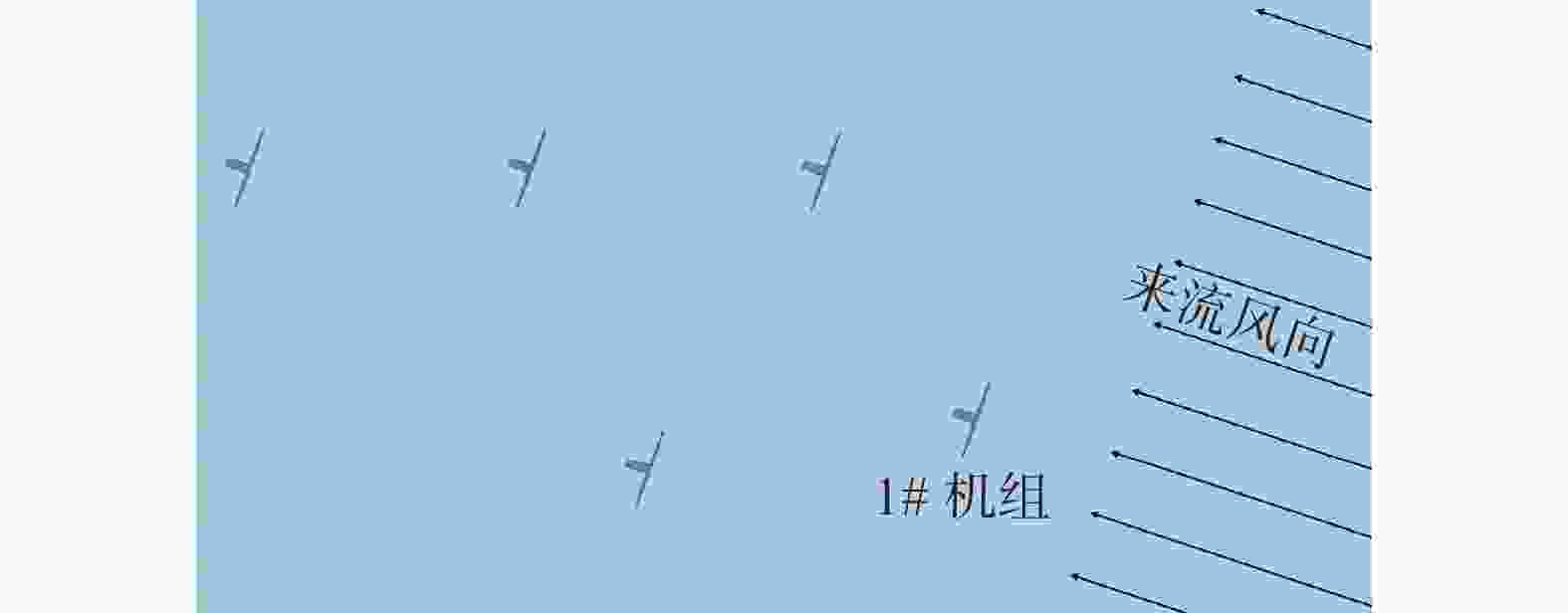
      Figure 3.  Location of wind turbine No. 1

      参数 工况1 工况2
      自由来流速度U0/(m·s−1) 5 11
      轮毂高度h/m 90 90
      风力叶轮直径D/m 112 112
      推力系数CT 0.800 0.574
      尾流膨胀系数k 0.4$ \times $I0 0.4$ \times $I0
      环境湍流强度I0 0.10 0.06

      Table 2.  Input parameters for case 1

    • 该数据为风洞实验数据,在米兰理工大学风洞实验室[24],采用G1级比例风力机进行实验,模拟2种不同湍流强度的速度流入,分别为中等湍流强度(I0=0.061)和高等湍流强度(I0=0.11),如图4所示。其来流风速分别为5.46 m/s、5.6 m/s。案例2的具体输入参数,如表3所示。

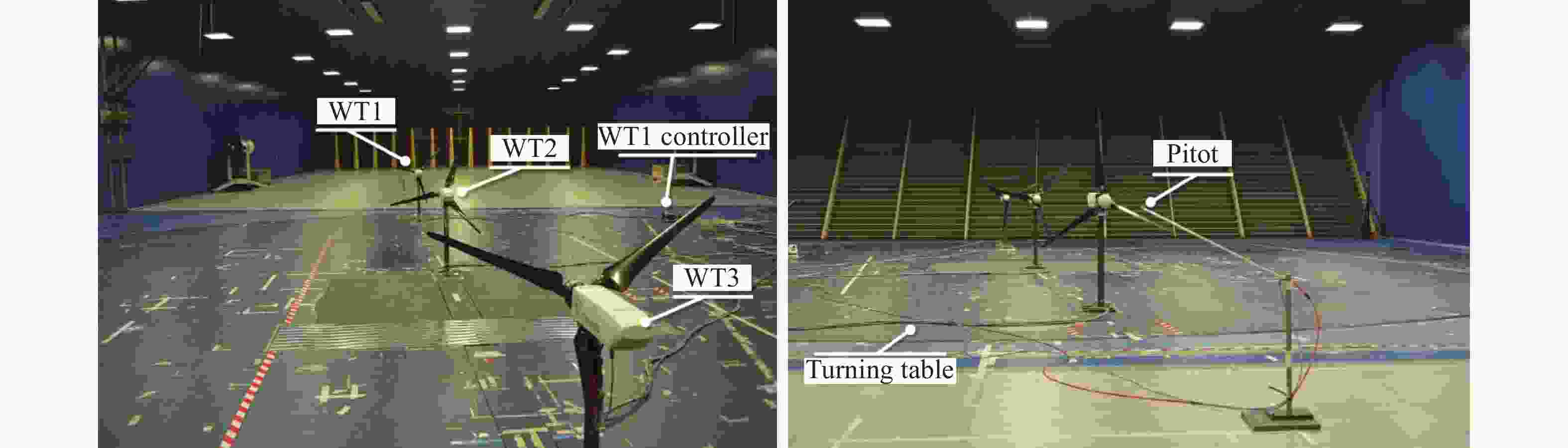
      Figure 4.  Wind tunnel test

      参数 数值
      自由来流速度U0/(m·s−1) 5.46/5.60
      风力叶轮直径D/m 1.1
      推力系数CT 0.68/0.69/0.79
      尾流膨胀系数k 0.4×I0
      环境湍流强度I0 0.061/0.100

      Table 3.  Input parameters for case 2

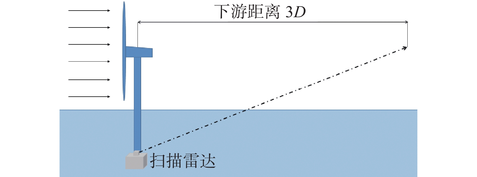
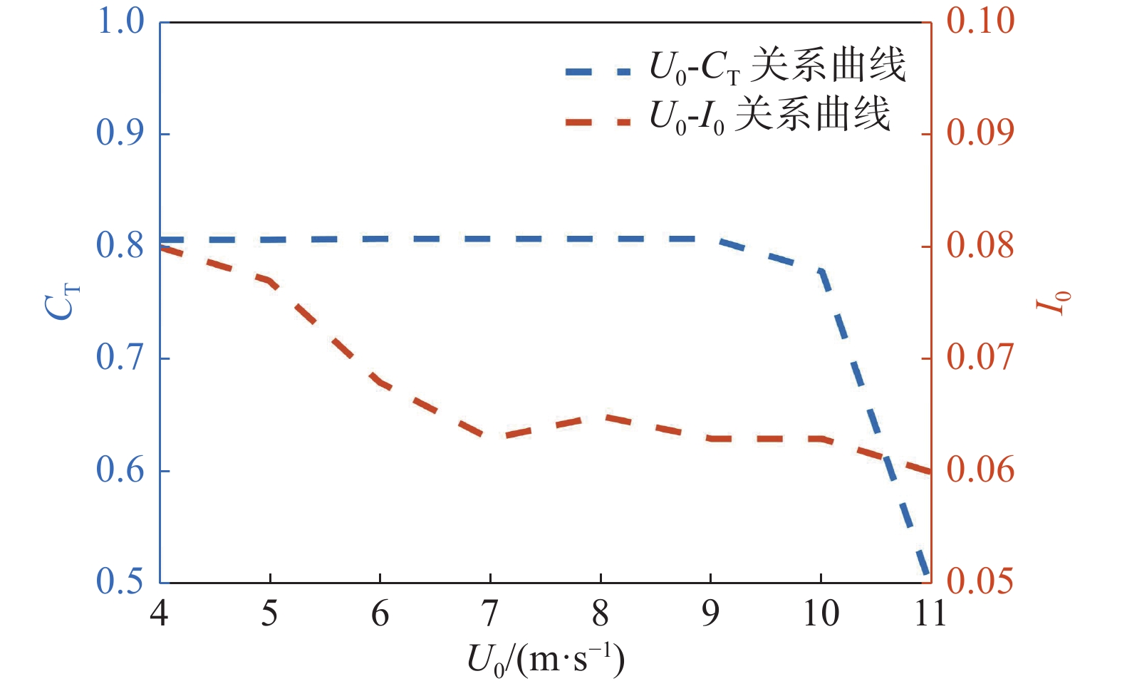
    • 该风场为海上风电项目,位于广东省。测试设备包含机舱雷达、扫描雷达各一台,机舱雷达位于机舱顶部向上游测量风场数据,用于得到环境风速及环境湍流强度。机组塔基3D雷达扫描模式为定向LOS模式,以连续采集海上风电机组下游3D距离轮毂高度处的风场数据,如图5所示,并计算其尾流湍流强度值。稳定观测时段为2022年11月~12月,场内风速多分布于4~11 m/s区间,观测机组为主风向下第一排机组,无机组尾流相互影响。案例3基本情况如表4所示,其中环境风速与推力系数及环境湍流强度的对应关系如图6所示,图中推力系数取机组当地空气密度下风速对应理论值。

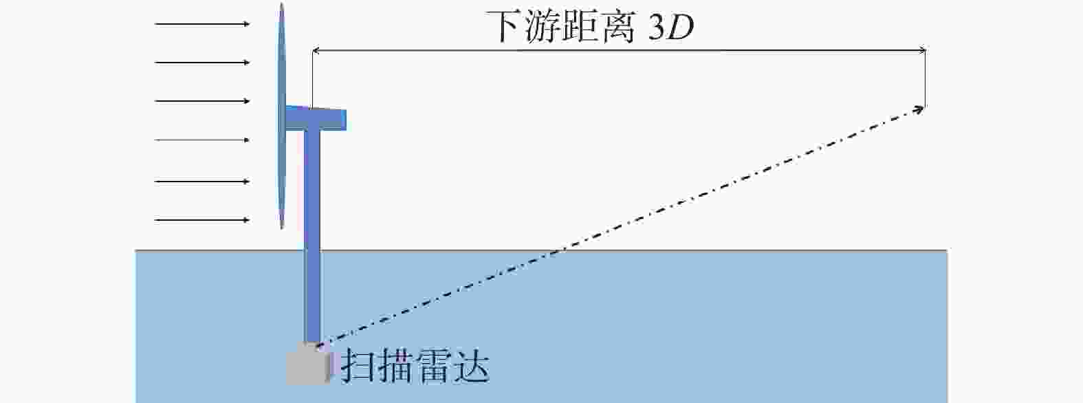
      Figure 5.  Directional LOS mode for 3D scanning radar

      参数 数值
      自由来流速度U0/(m·s−1) 4~11
      轮毂高度h/m 108
      风力叶轮直径D/m 158
      尾流膨胀系数k 0.4$ \times $I0

      Table 4.  Input parameters for case 3

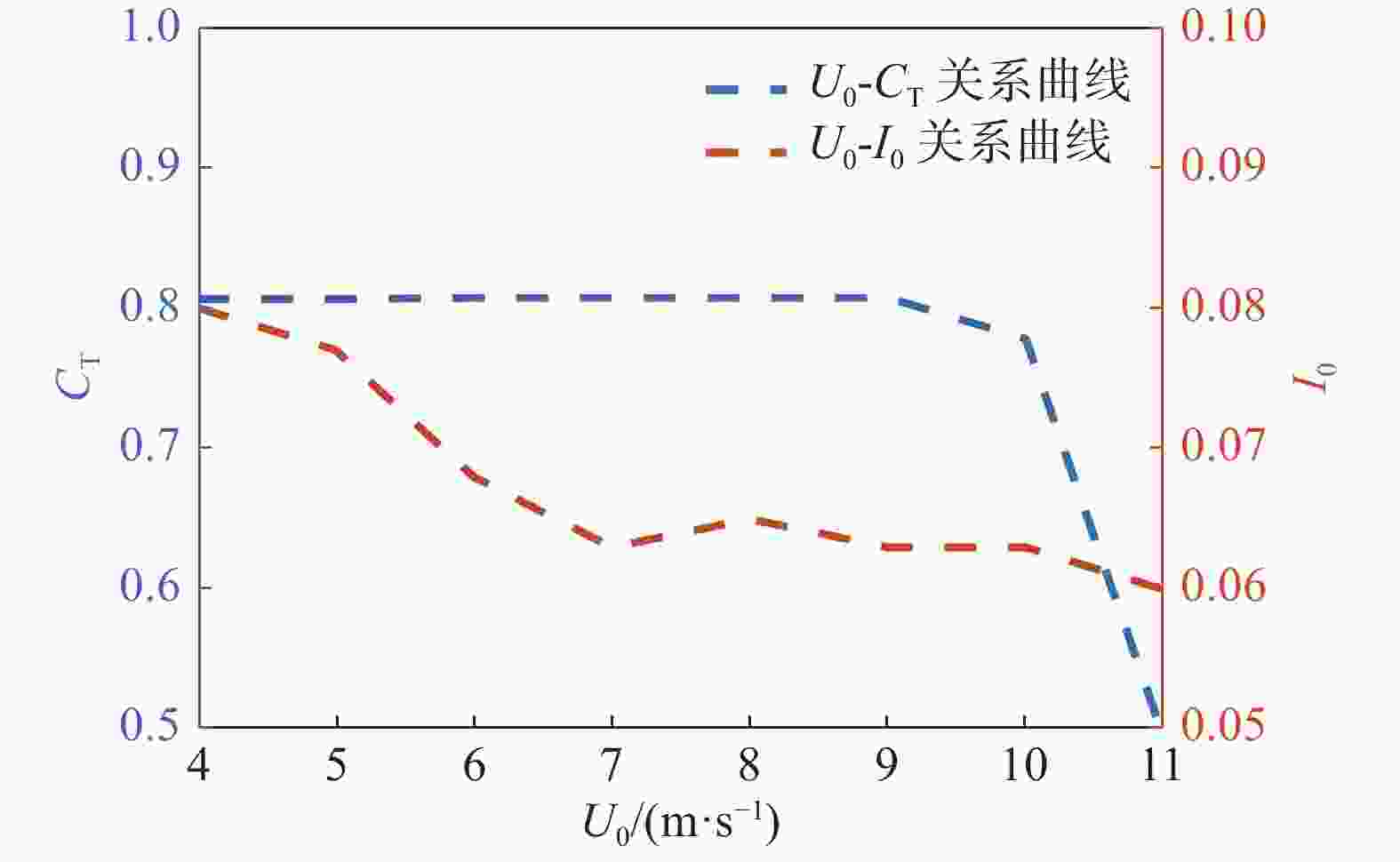
      Figure 6.  Correspondence of ambient wind speeds with thrust coefficient and ambient turbulence intensities

    • 为精准评估各尾流模型预测性能,确保评估结论的合理性,本文将以尾流模型输出的预测结果与对应实验结果的偏差[27]、平均偏差及偏差标准差为评定因子,定量分析各尾流模型预测表现,考虑实际风场上下游机组距离一般处于[3D,10D]范围内,因此各模型的对比研究将在该范围内进行。偏差、平均偏差及偏差标准差的计算公式如下:

      $$ \delta (\mathrm{\%})=\frac{\left|{U}_{{\rm{model}}}-{U}_{{\rm{exp}}}\right|}{{U}_{{\rm{exp}}}}\times 100\mathrm{\%} $$ (41)
      $$ \stackrel-{\delta }(\mathrm{\%})=\frac{\sum _{i=1}^{i=n}\delta (\mathrm{\%})}{n} $$ (42)
      $$ {\delta }_{{\rm{std}}}(\mathrm{\%})=\frac{\sqrt{\sum _{i=1}^{i=n}{(\delta (\mathrm{\%})-\stackrel-{\delta }(\mathrm{\%}))}^{2}}}{n} $$ (43)

      式中:

      $ \delta $ ——数据偏差;

      $ {U}_{{\rm{model}}} $ ——尾流模型预测速度(m/s);

      $ {U}_{{\rm{exp}}} $ ——相关实验探测的速度值(m/s);

      $ \stackrel{-}{\delta } $ ——偏差平均值;

      n ——偏差计算范围内的实验值数量;

      $ {\delta }_{{\rm{std}}} $ ——偏差标准差。

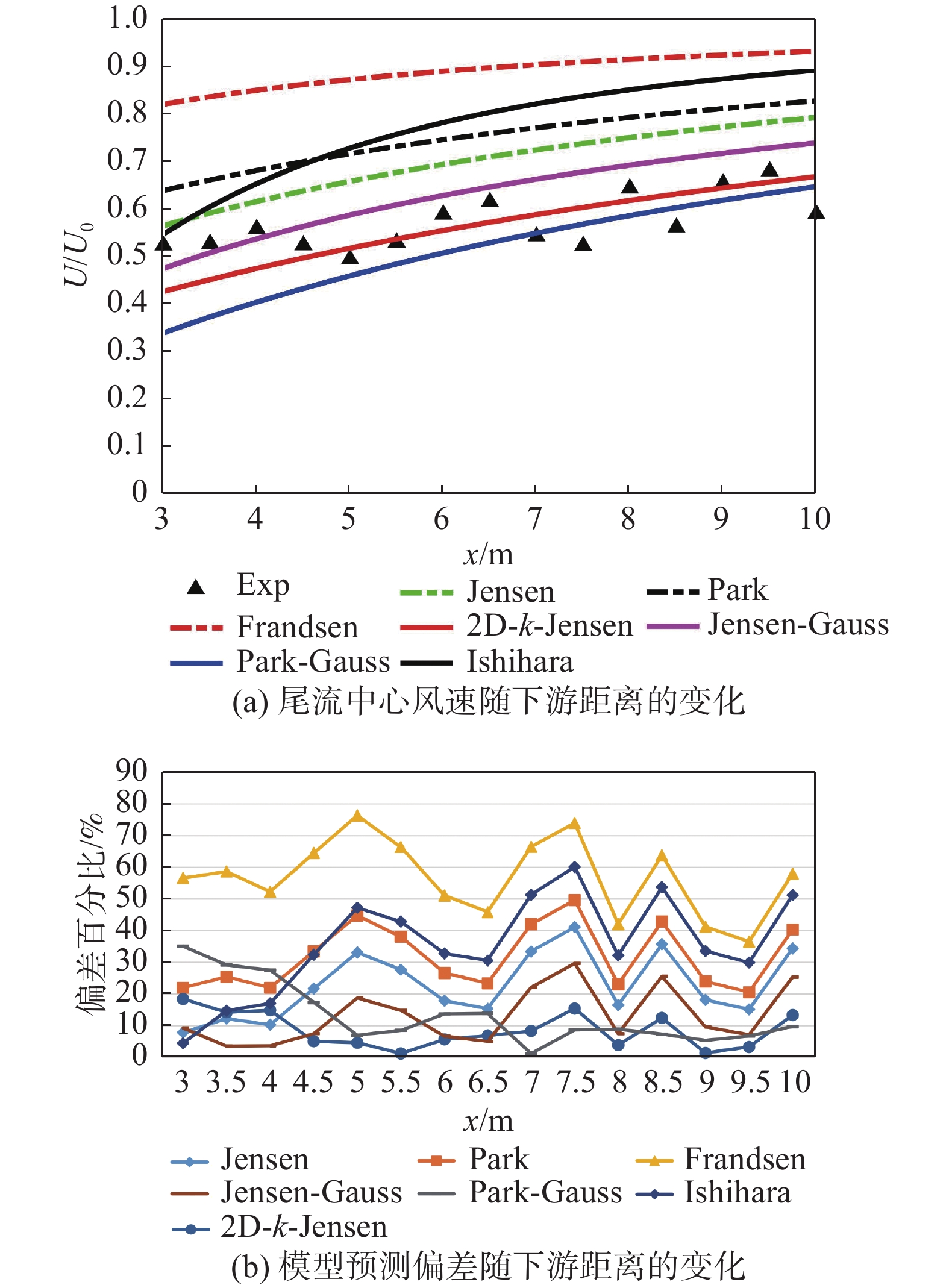
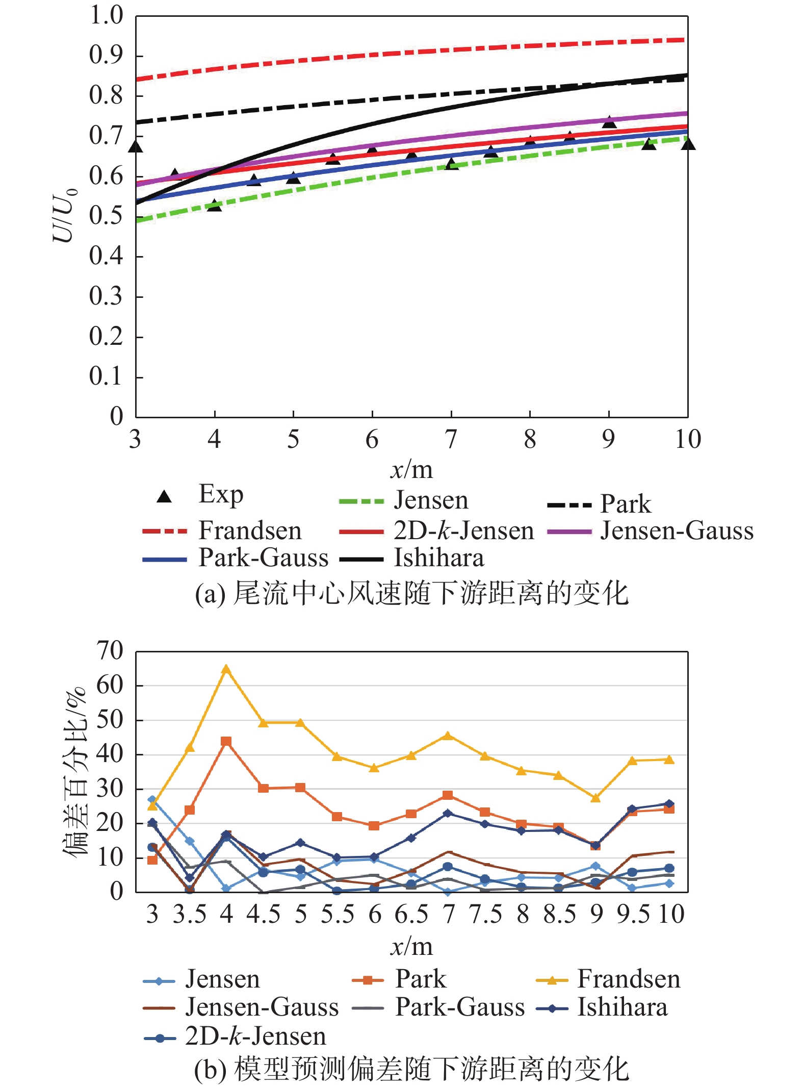
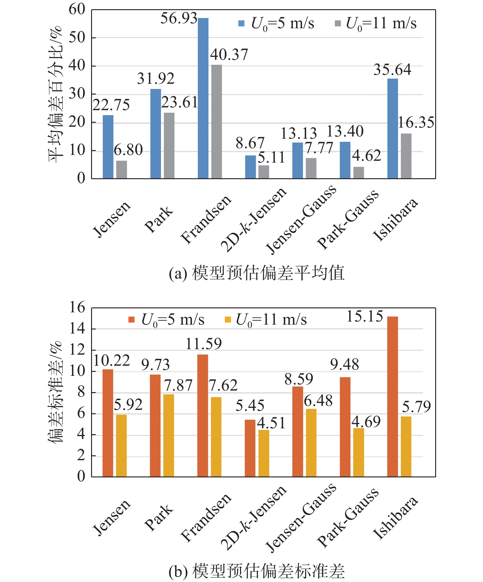
    • 为分析各尾流模型风速预测性能,采用案例1和案例2数据来计算预测值与实验值的偏差。案例1数据为海上风场,采用2种风速下(5 m/s、11 m/s)的尾流数据,分析环境风速变化下各模型的预测性能,如图7~图9所示。大多数模型的预测偏差随下游距离的变化趋势大体一致且偏差波动较为稳定,图7图8图9(b)也进一步量化表明了各模型除Frandsen和Ishihara在5 m/s风速工况以外,在下游区域3D~10D均有着较为稳定的风速预测。对于上下游机组间距最可能出现范围(5D~7D),仅有2D-k-Jensen在两组风况下满足偏差低于10%,Jensen、Jensen-Guass和Park-Guass仅在11 m/s环境风速下能实现较好的预测精度。对比不同风速下各模型预估偏差的平均值与标准差来看,如图9所示,高风速工况下,各模型均能获得一个更优的尾流风速预测精度和适应性,即模型预估偏差的平均值与标准差更小。当环境风速为5 m/s时,仅2D-k-Jensen出现了较为精准的预测,平均偏差约9%,而在11 m/s环境风速下,Jensen、2D-k-Jensen、Jensen-Guass和Park-Guass均有着更优的预测情况,偏差平均值及标准差均低于8%,其中Jensen为唯一的一维模型,这与文献[27]结论一致。

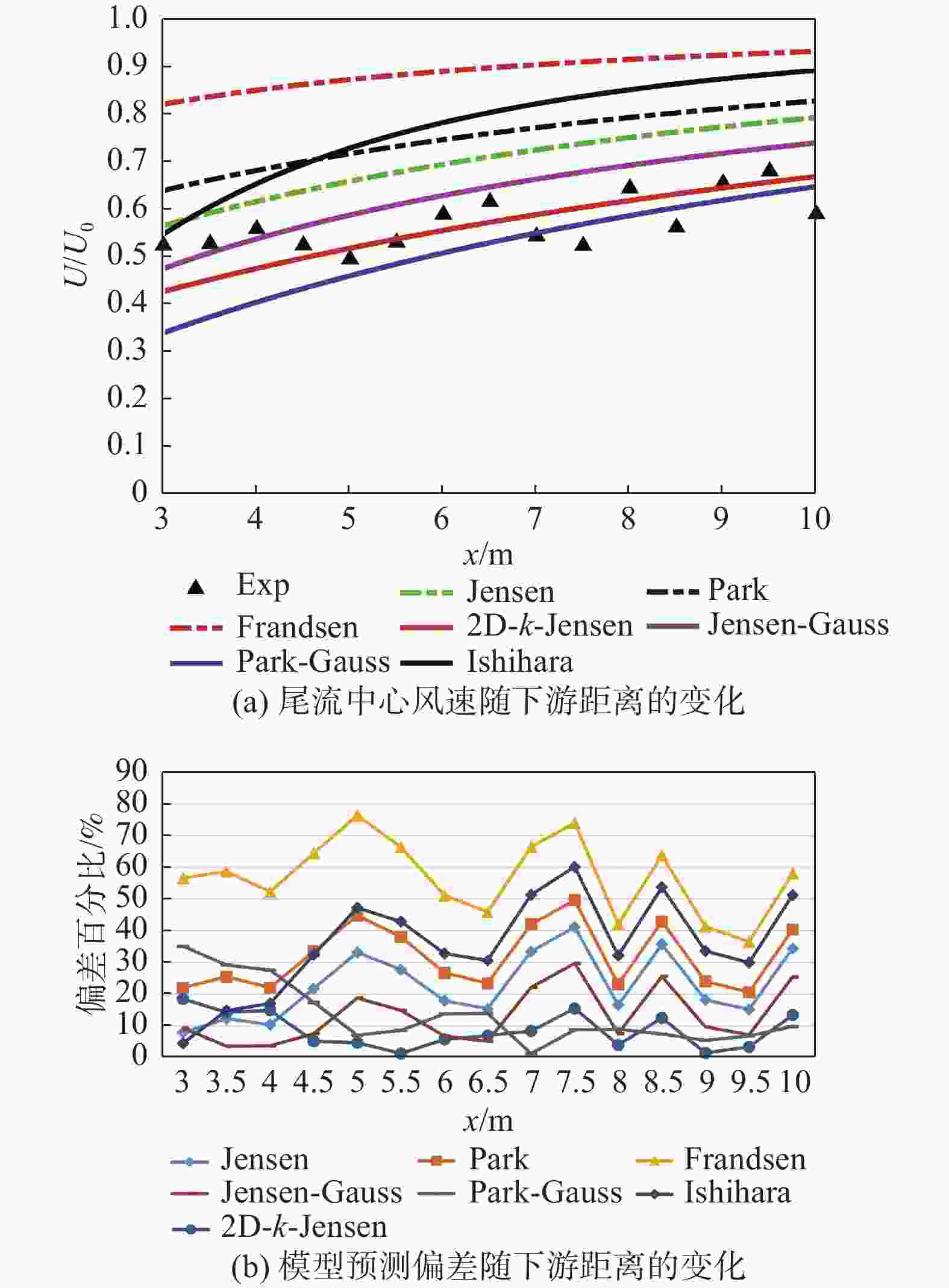
      Figure 7.  Comparison of wind speed predictions from models with experimental values, U0=5 m/s(case 1)

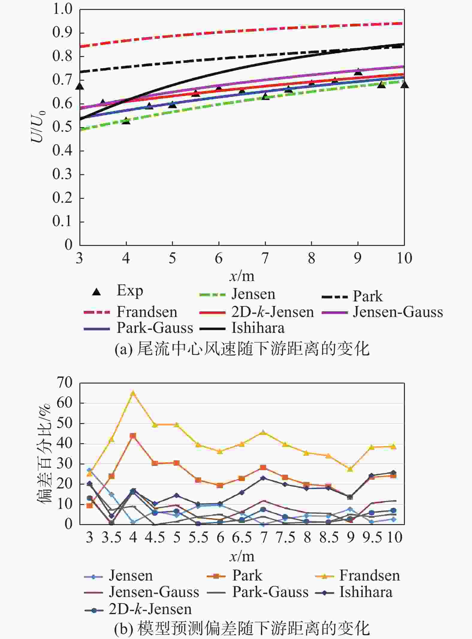
      Figure 8.  Comparison of wind speed predictions from models with experimental values, U0=11 m/s(case 1)

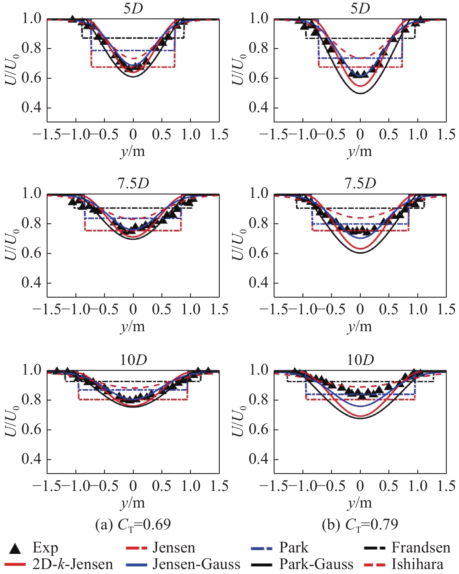
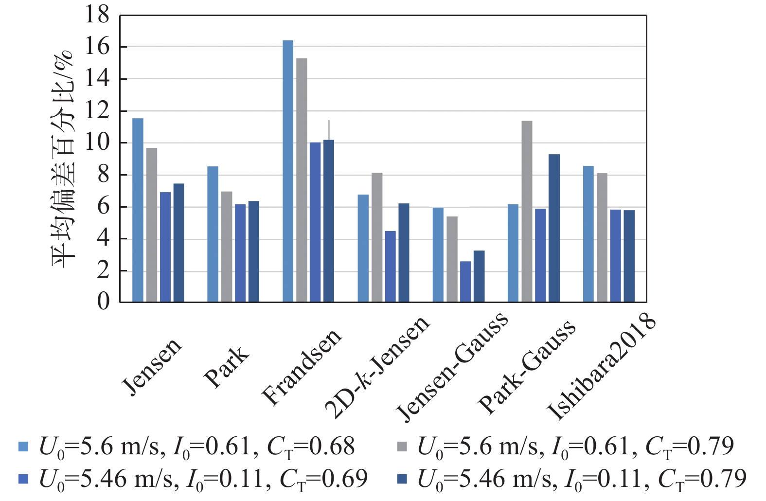
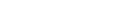
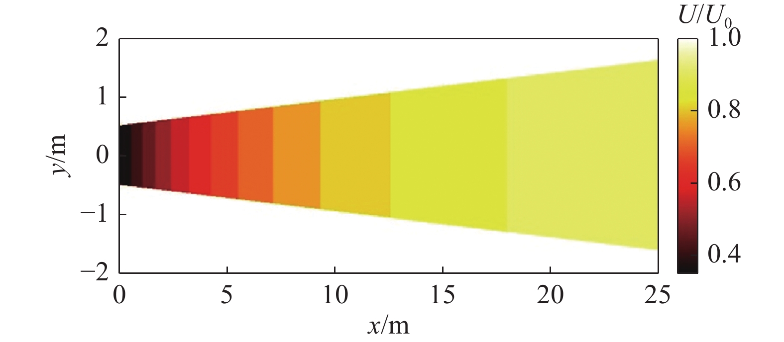
      相较于案例1的研究重点在尾流中心风速的预估分析,案例2主要关注各预测模型在轮毂高度处水平面(XY截面)的水平风速分布预测情况,实验值与模型预估值对比结果如图10~图12所示。图10图11显示风机尾流水平分布呈高斯型,与二维尾流预估模型形状更为契合。Ishihara模型风速预测更高且尾流宽度更宽,而2D-k-Jensen、Park-Guass则反之,相较之下Jensen-Guass模型在各工况与实验值的贴合度更高。对于一维模型,多组工况中Jensen模型对尾流中心的风速预测均优于Park和Frandsen等一维模型,但因其恒定的下游尾流分布,尾流中心风速预测更佳的Jensen模型在各工况下的预估平均偏差均高于Park模型,如图12所示。结合各工况结果,Park、2D-k-Jensen、Jensen-Guass和Ishihara模型在各工况下均有着较优的预测性能,平均偏差小于9%。同时,高环境湍流工况下,各模型的预测性能均有略微提升。

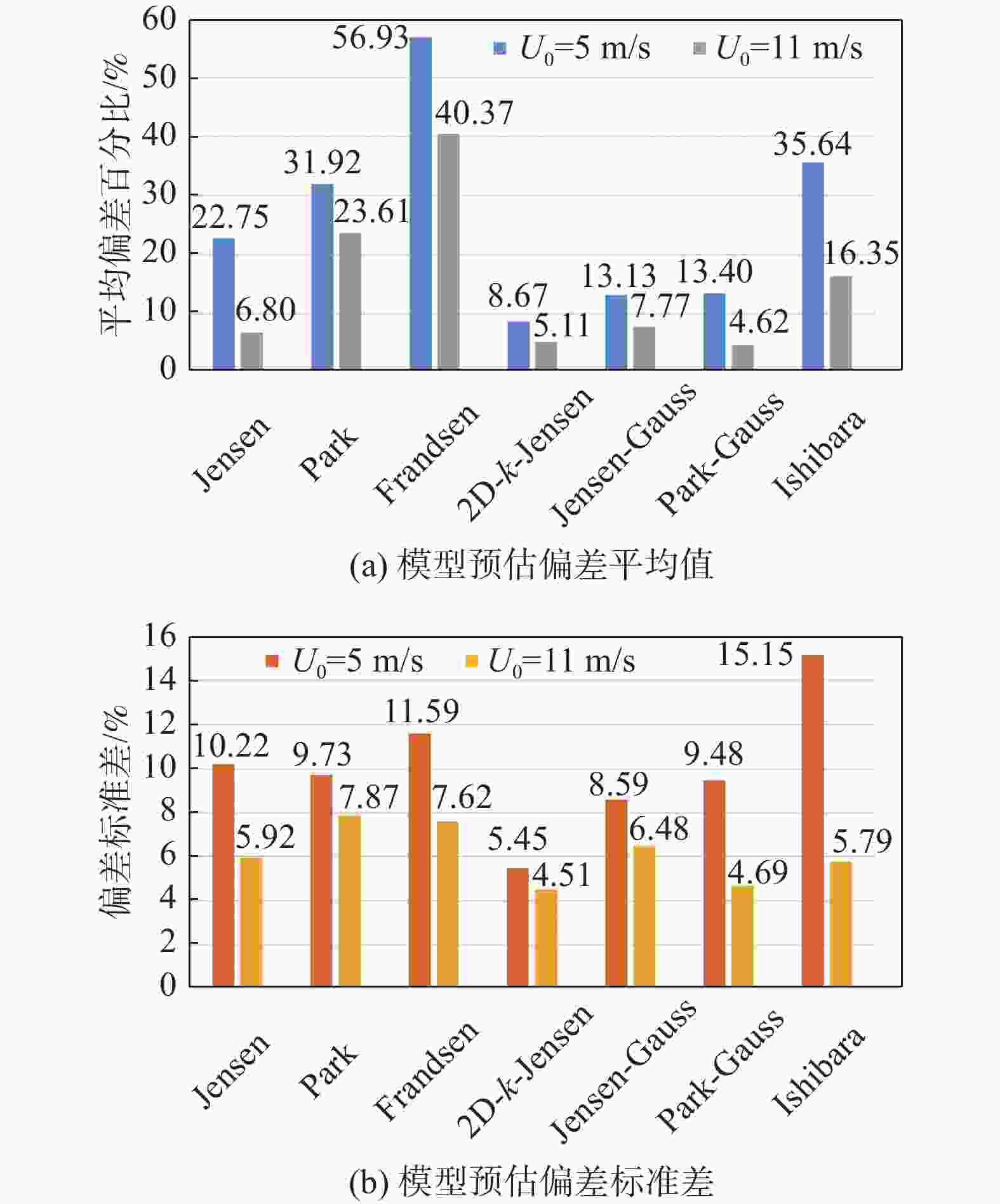
      Figure 9.  Mean and standard deviation of wind speed prediction deviations from models(case 1)

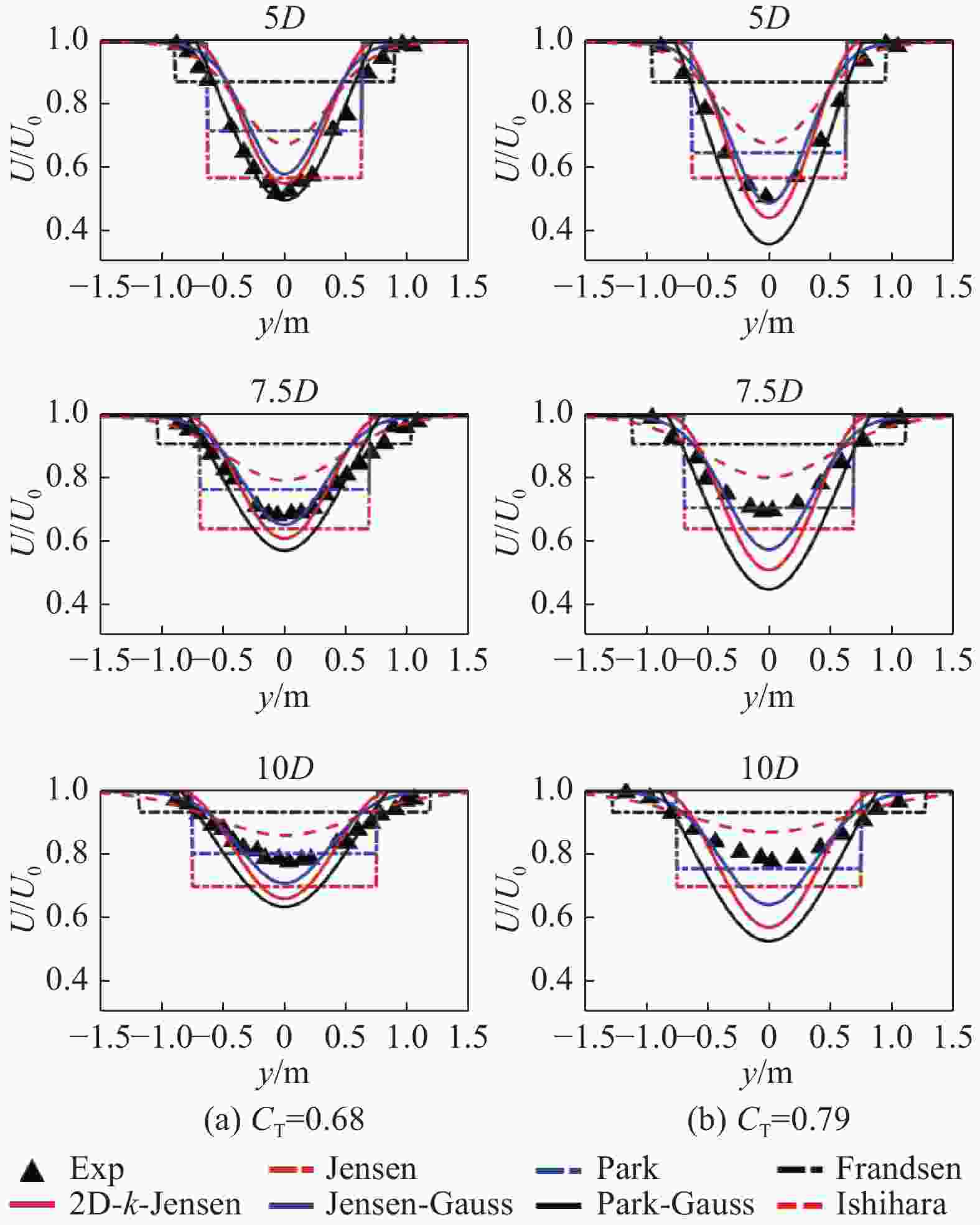
      Figure 10.  Comparison of wind speed predictions from models with experimental values, U0=5.6 m/s、I0=0.061(case 2)

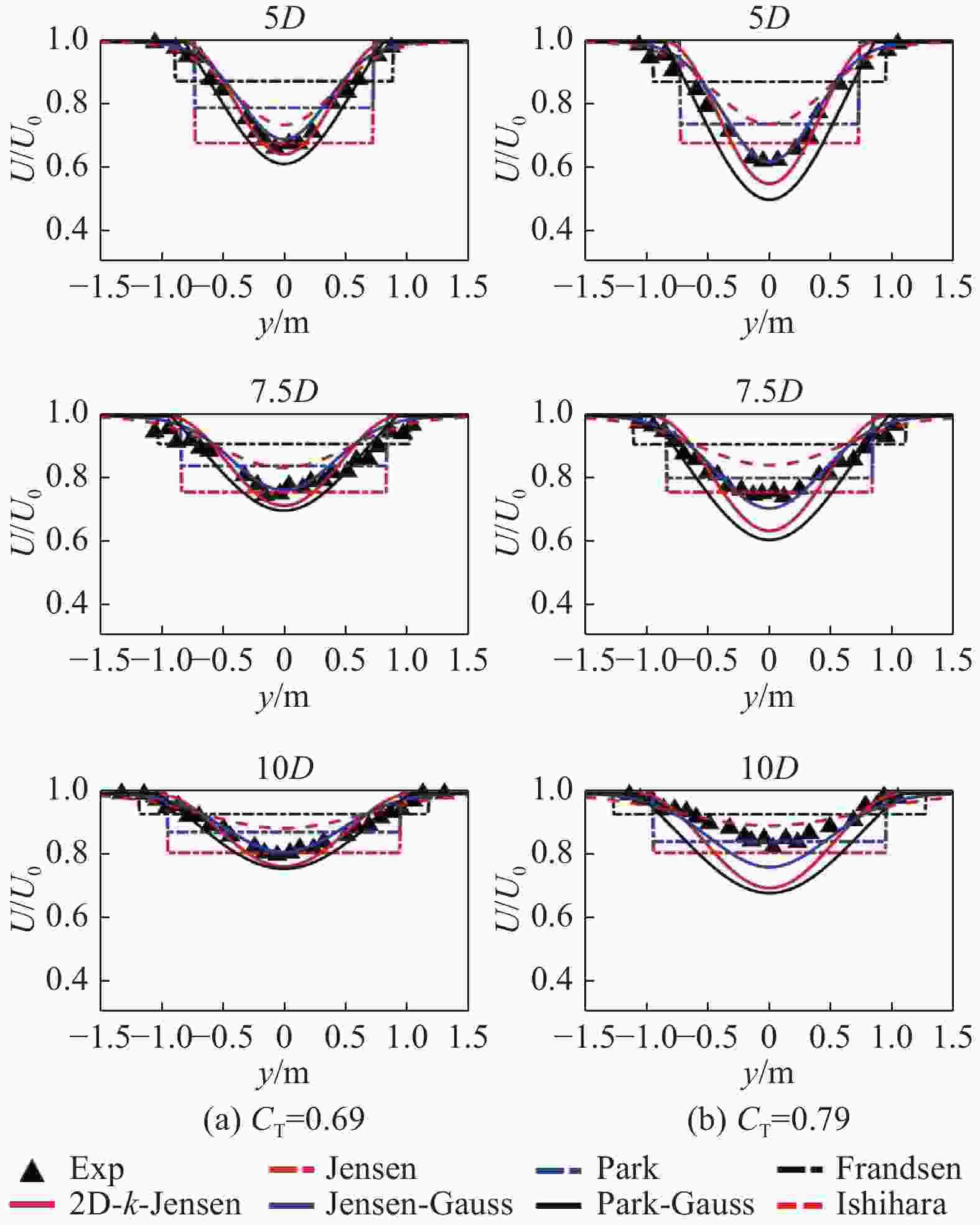
      Figure 11.  Comparison of wind speed predictions from models with experimental values, U0=5.46 m/s、I0=0.11(case 2)

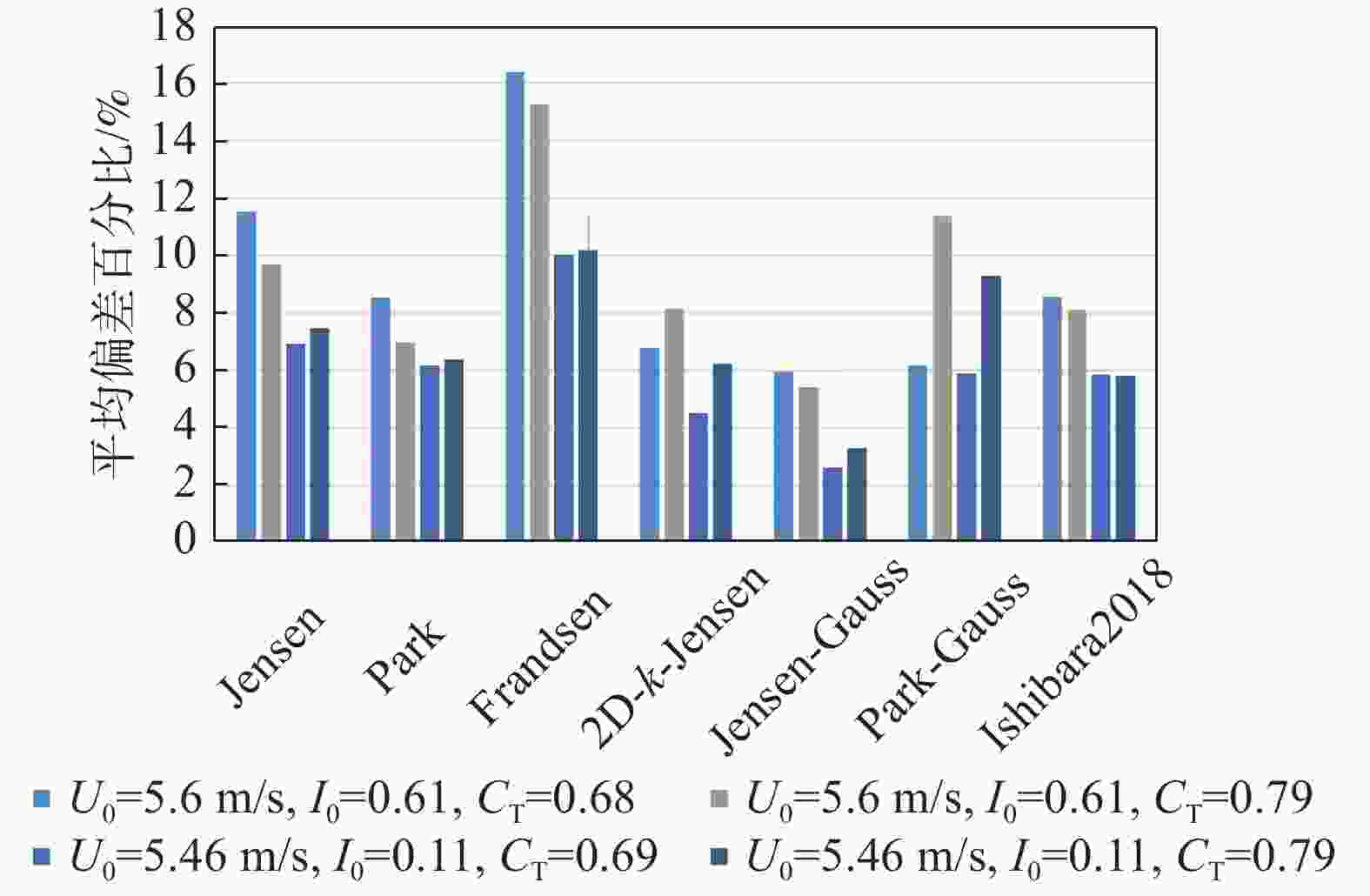
      Figure 12.  Mean percentage deviation of wind speed predictions from models(case 2)

      结合两组案例数据分析结果来看,针对不同的环境条件,模型的风速预测性能有一定变化,高上游风速工况下,各模型预估精度及稳定性均有明显提升,同时环境湍流强度的提升也对模型预测精度也有着略微的改善作用。二维尾流模型风速预估精度普遍优于一维尾流模型,Ishihara较实验值预测出更快的尾流风速恢复,不适用于机组尾流风速预估,而Jensen-Guass、2D-k-Jensen、Park-Guas则与实验结果较为接近,三者最大平均偏差分别为13.4%、8.7%、13.1%,其中前两者因其可变的尾流膨胀系数有着更优的预测特点,Jensen-Guass尾流宽度预测更佳,而2D-k-Jensen尾流中心风速预测精度更高且多工况适应性更强,最大偏差标准差低于6%,均适用于机组尾流风速损失的预估。一维尾流模型中,虽Jensen模型尾流中心风速预估精度远优于Park、Frandsen模型,但风速水平分布预测上略差于Park模型,相较于前者,Park模型更适用于机组尾流风速预测。

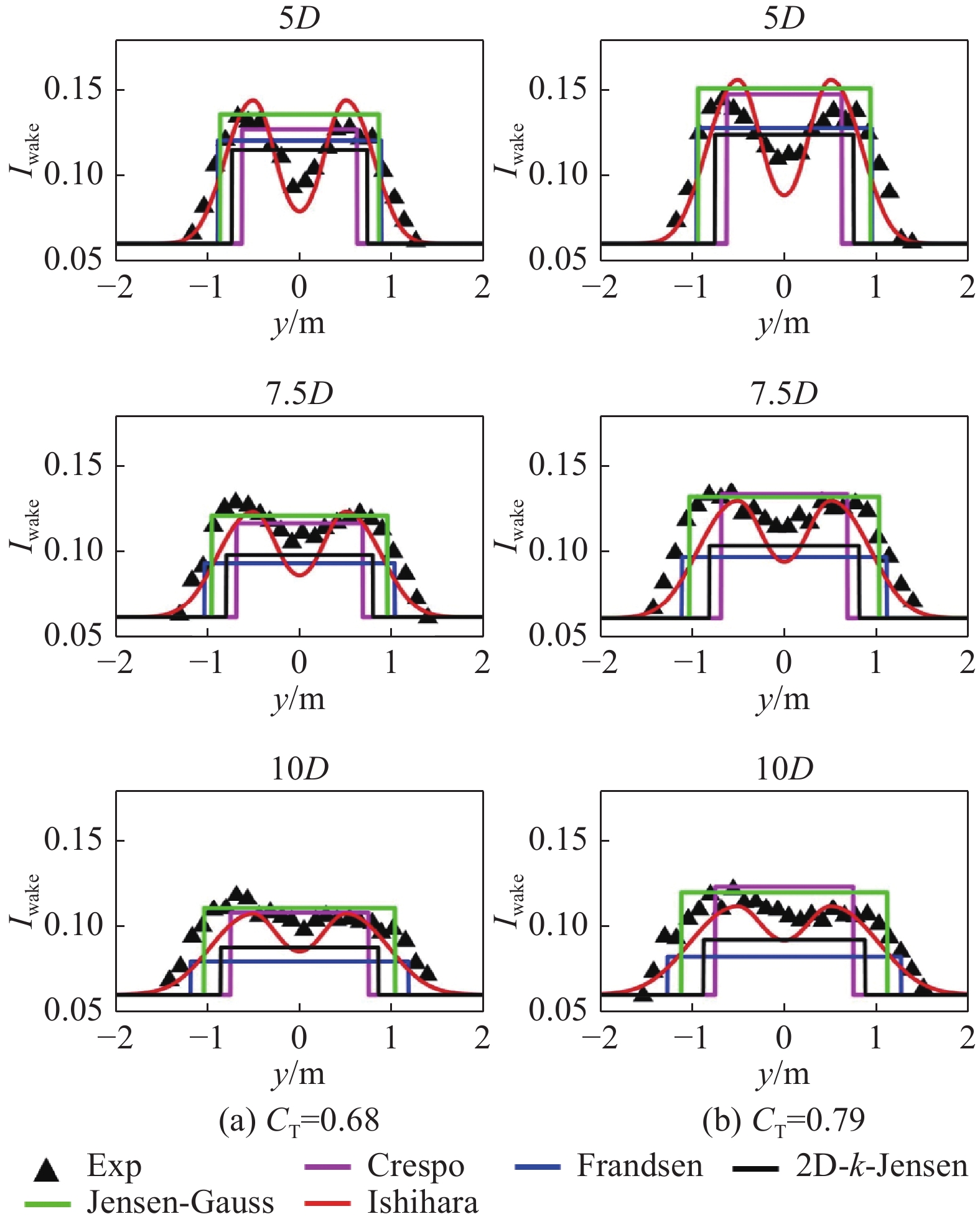
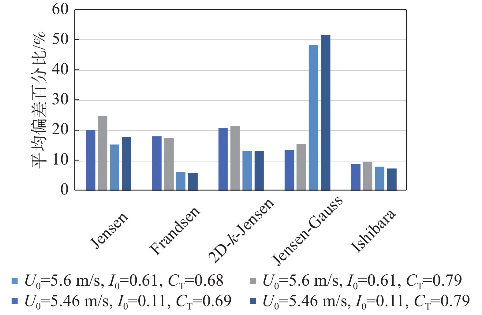
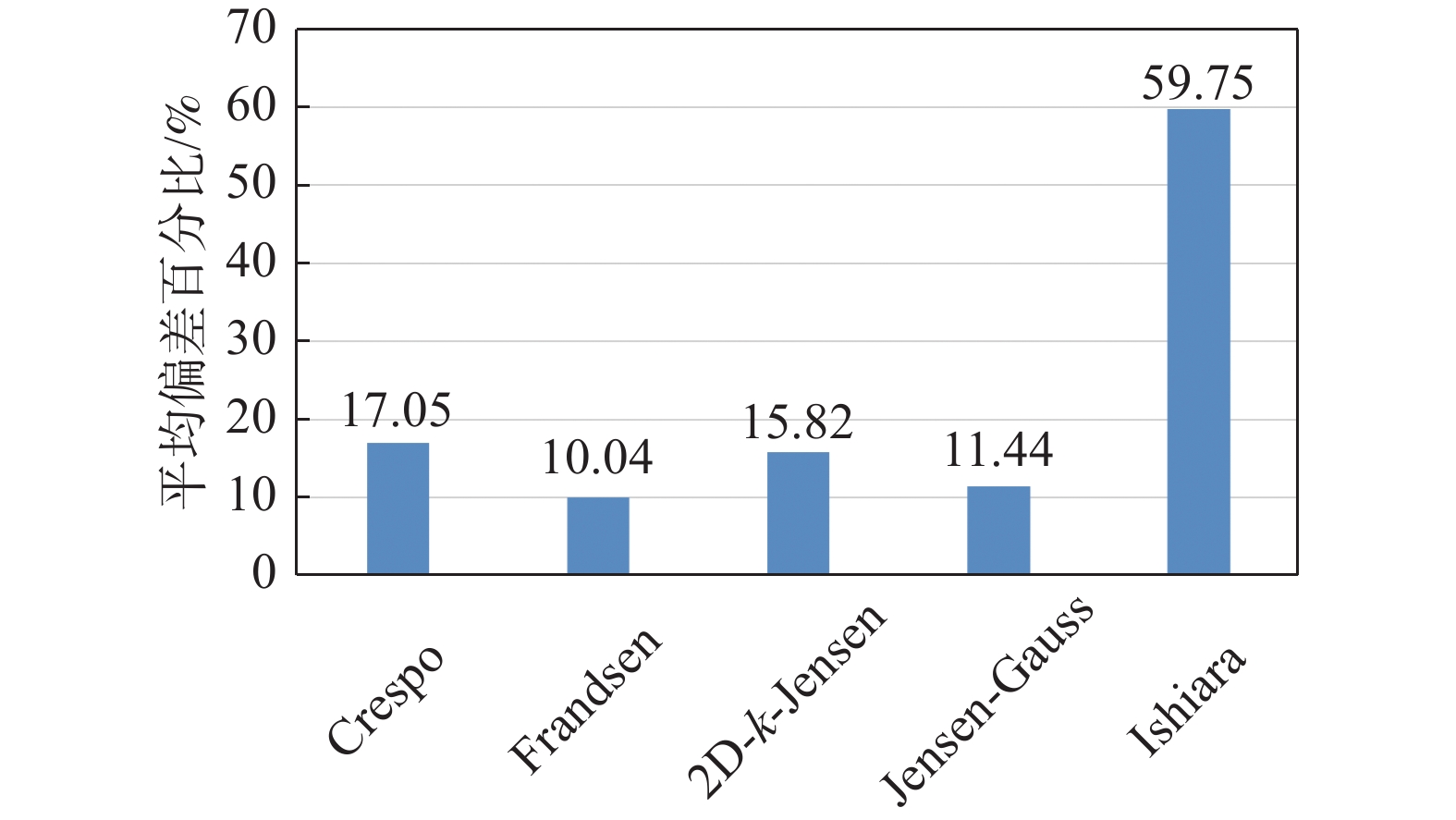
    • 利用案例2和案例3中机组尾流湍流强度相关数据评估各尾流模型的湍流强度预测性能及适用性。图13~图15基于案例2数据展现了机组尾流不同下游距离湍流强度的水平分布对比情况。机组尾流湍流强度水平分布呈“双驼峰状”与Ishihara预测的双高斯形较为接近。对于低湍流强度时,各模型预测结果均与实验值较为接近,而Jensen-Guass模型在高湍流强度工况下预测出远大于实验的湍流强度结果,平均偏差约50%,对环境湍流强度变化极为敏感。根据图15平均偏差结果显示,除Jensen-Guass模型以外,其余模型高湍流强度工况预测结果均优于低湍流强度,其中Frandsen模型差异最为明显,而Ishihara模型则相反,两组工况预测精度接近,平均偏差均小于10%。

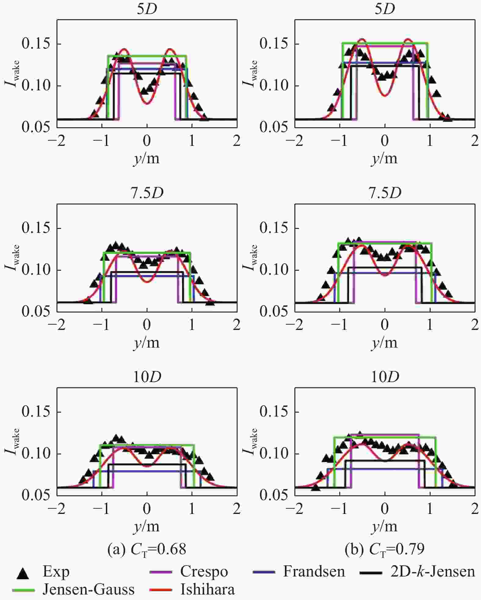
      Figure 13.  Comparison of turbulence intensity predictions from models with experimental values, U0=5.6 m/s、I0=0.061(case 2)

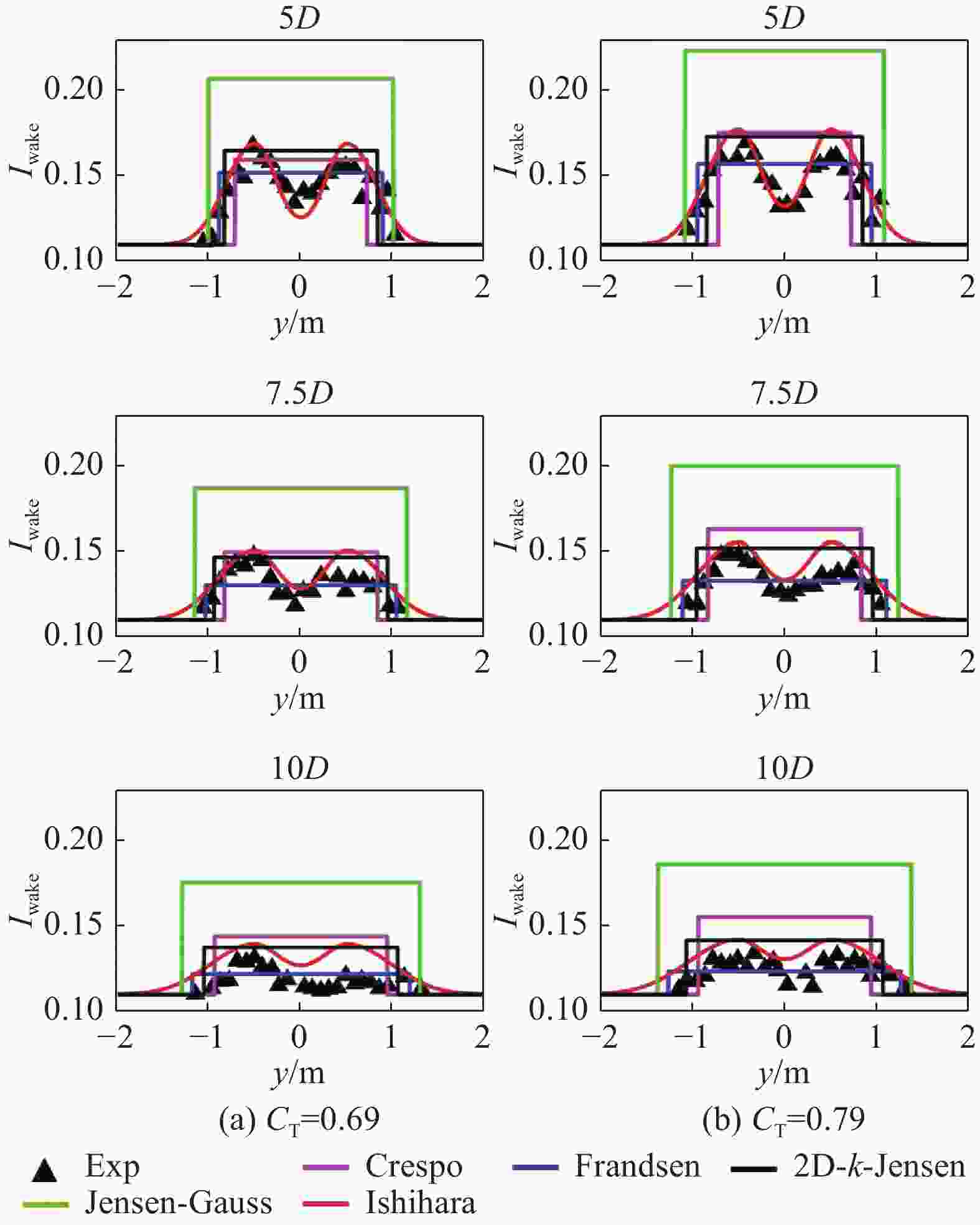
      Figure 14.  Comparison of turbulence intensity predictions from models with experimental values, U0=5.46 m/s、I0=0.11(case 2)

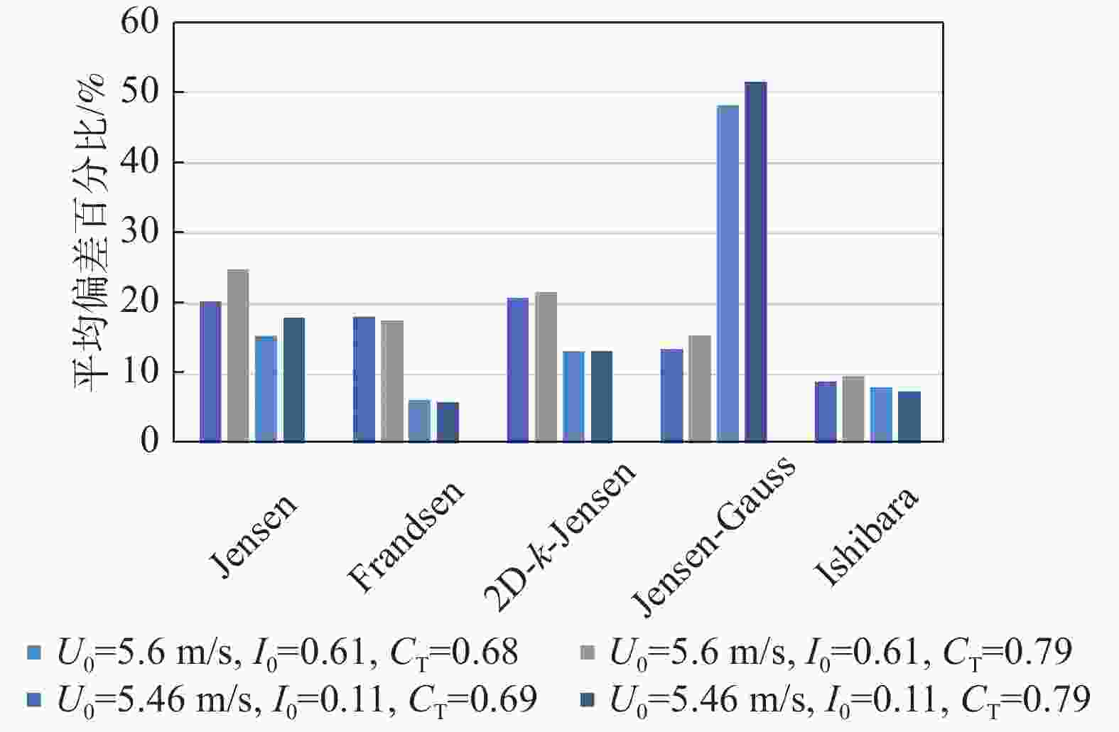
      Figure 15.  Mean percentage deviation of turbulence intensity predictions from models(case 2)

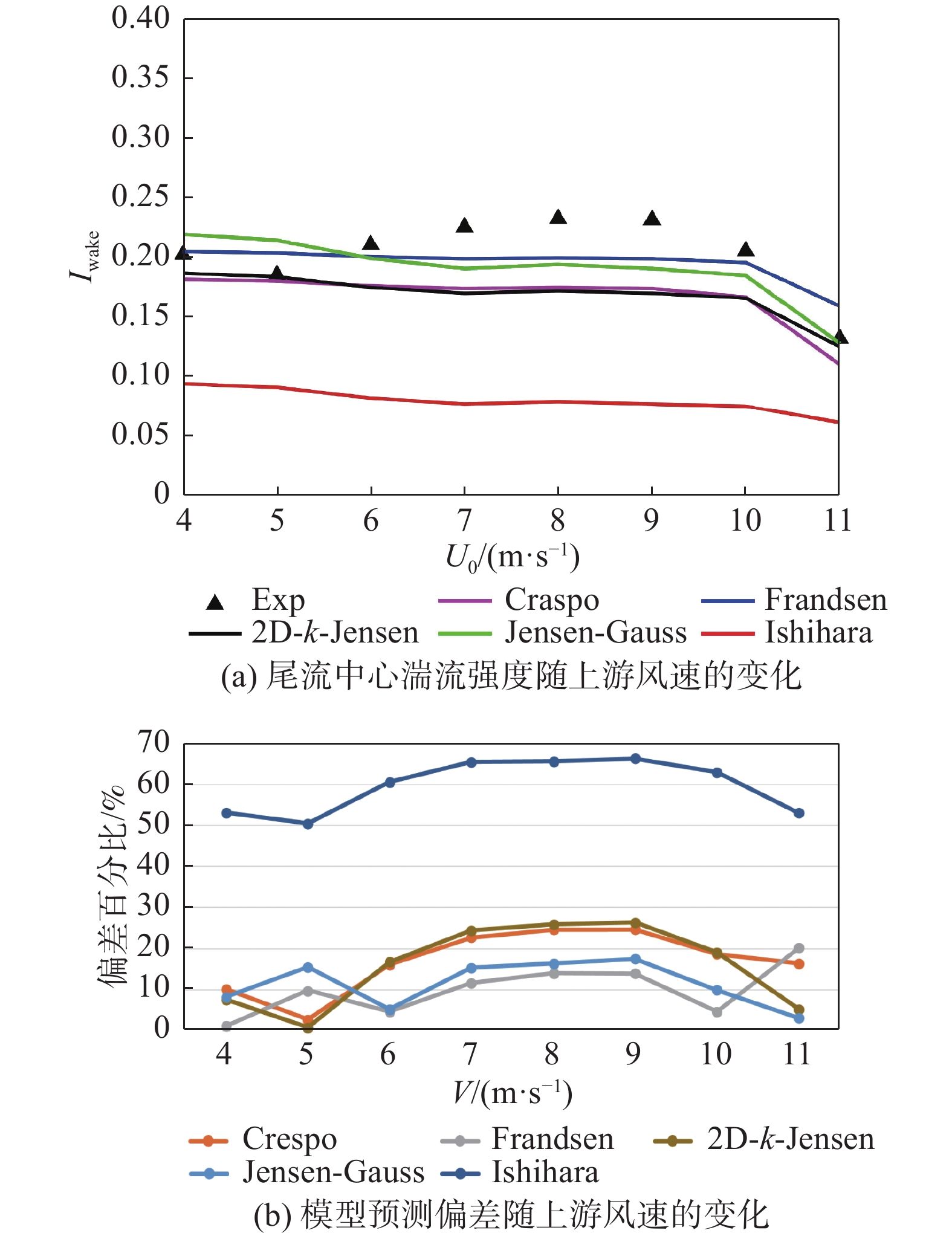
      案例3中的所有实验数据均为下游恒定距离3D处的湍流强度值,用于分析上游风速变化下模型预测的偏差情况。图16展示了各湍流强度预估模型与实验值的数值对比及相应偏差。除Ishihara以外的模型预测偏差相差不大,Ishihara因其具有的双高斯形状,导致尾流中心湍流预测值远低于实验值。上游风速6~10 m/s范围,各模型预估数值均低于实验值情况,其中Frandsen预估相对最好,但在7~9 m/s范围的偏差仍超过10%。上游风速为11 m/s时,Jensen-Guass、2D-k-Jensen有着约5%的较小预测偏差。根据不同上游风速各模型预测的平均偏差结果,如图17所示,仅Frandsen模型有着可接受的平均偏差值,约为10%。

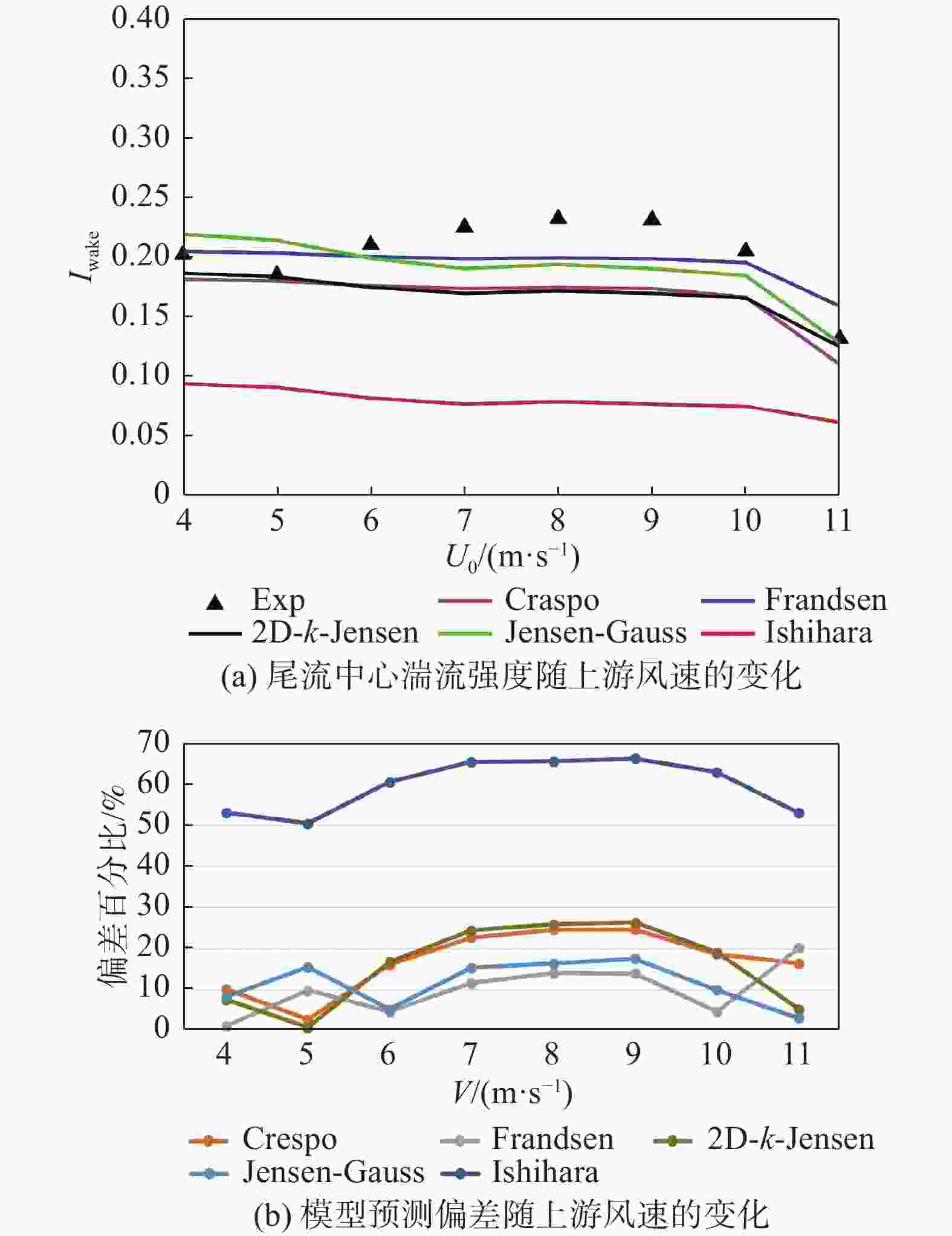
      Figure 16.  Comparison of turbulence intensity predictions from models with experimental values(case 3)

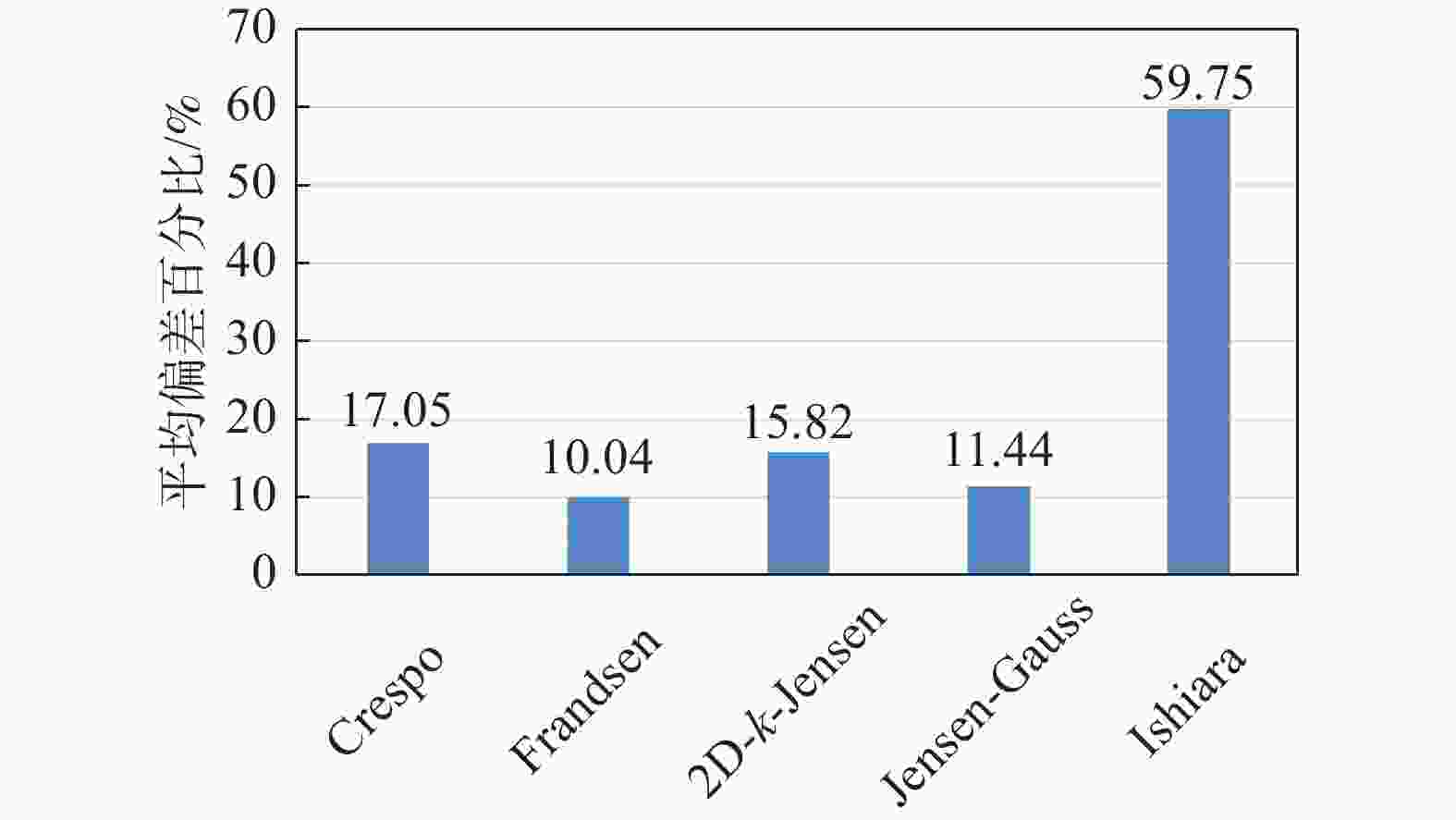
      Figure 17.  Mean percentage deviation of turbulence intensity predictions from models(case 3)

      综合案例2和案例3湍流强度预测的分析情况,各尾流模型在机组尾流湍流强度预测的性能上也存在着明显的共性,即高湍流强度模型预估精度将有所提升,Jensen-Guass模型除外。Jensen-Guass模型预测结果极不稳定,高环境湍流强度下预估出远高于实验值的结果,平均偏差约50%。虽Ishihara模型在湍流强度水平分布预测上展现出明显的优势,预估平均偏差均低于10%,但其尾流中心处的湍流强度预测结果远低于实测值,平均偏差约60%,不利于预估下游机组处湍流强度值。其余模型在两案例中的湍流强度预估平均偏差相差不大,其中Frandsen模型预测精度及稳定性相对最好,大多工况平均偏差低于10%。

    • 本文对常见的8个机组尾流模型进行了系统的研究,依托3组风场实测或风洞实验数据,着重分析了各模型尾流风速和湍流强度的预估情况,主要结论如下:

      1)尾流速度预测分析所考察的模型中,尾流膨胀系数k可变的Jensen-Guass及2D-k-Jensen模型能较好地反应尾流速度分布情况,风速预估结果与实测值吻合较好,均适用于机组尾流风速损失的预估。WT/WASP等商业软件常用的一维Park模型,也展现出不错的预估性能。Ishihara模型风速预估虽通过更多更复杂的参数进行构建,但预测结果不太理想。

      2)对于湍流强度预测方面,Jensen-Guass模型对环境湍流强度变化敏感,预测结果极不稳定,Ishihara模型无法精准预测下游机组位置处湍流强度,需对尾流中心处湍流强度预测进行调整,其余模型预测结果差异较小,Frandsen模型预测精度及稳定性相对最好,适用于机组尾流湍流强度预估。

      本文基于单机组尾流研究各尾流模型预估性能,可为海上风场机位排布优化及尾流控制分析的尾流模型选择做参考。后续将根据现有结果优化单尾流模型,并结合多尾流叠加理论,进一步讨论各模型针对整场尾流损失的预测表现。

Reference (27)

Catalog

    /

    DownLoad:  Full-Size Img  PowerPoint
    Return
    Return